
| Basic Research | https://doi.org/10.21041/ra.v15i3.784 |
Virtual determination of displacements in bell towers of historical buildings subjected to seismic actions and subsidence, using shell elements, linear dynamic analysis, and modified linear analysis. Case study: Temple of Santa Veracruz
Determinación virtual de desplazamientos en torres campanario de edificios históricos sometidos a acciones sísmicas y hundimientos, utilizando elementos shell, análisis dinámico lineal y lineal modificado. Caso de estudio: Templo de la Santa Veracruz
Determinação virtual de deslocamentos em torres sineiras de edifícios históricos sujeitos a acções sísmicas e subsidência, utilizando elementos de casca, análise dinâmica linear e linear modificada. Estudo de caso: Templo de La Santa Veracruz
C. A. Torres Montes de Oca1* , J. E. Rosas Valencia2
1 Research professor at Sección de Estudios de Posgrado e Investigación (SEPI), Escuela Superior de Ingeniería y Arquitectura Unidad Tecamachalco (ESIA UT), Instituto Politécnico Nacional (IPN), 53950, Naucalpan de Juárez, Estado de México, México, http://www.sepi.esiatec.ipn.mx.
2 Master's degree student at Escuela Superior de Ingeniería y Arquitectura Unidad Tecamachalco (ESIA UT), Instituto Politécnico Nacional (IPN), 53950, Naucalpan de Juárez, Estado de México, México, http://www.esiatec.ipn.mx.
*Contact author: ktcate2@hotmail.com; ctorresmo@ipn.mx
Received: 25/10/2024
Revised: 02/06/2025
Accepted: 05/08/2025
Published: 01/09/2025
| Cite as: Torres Montes de Oca, C. A., Rosas Valencia, J. E. (2025), “Virtual determination of displacements in bell towers of historical buildings subjected to seismic actions and subsidence, using shell elements, linear dynamic analysis, and modified linear analysis. Case study: Temple of Santa Veracruz”, Revista ALCONPAT, 15 (3), pp. 249 – 298, DOI: https://doi.org/10.21041/ra.v15i3.784 |
Abstract
The objective of this work is to analyze the behavior of the bell towers of a historical heritage temple built with irregular masonry, it is analyzed by means of a finite element model of shell types and turning blocks. The results showed a coherent relationship of the behavior with respect to section changes. Differential subsidence drastically increased the displacements. One limitation was the interruption of access, due to intervention activities in the building. The uniqueness of this work is based on the graphic superposition of the displacements calculated for different combinations of isolated and combined actions. In conclusion, the displacements obtained with time signals are less critical than those determined with response spectrum.
Keywords: bell towers, differential subsidence, dynamic analysis, modified linear analysis, historic buildings.
1. INTRODUCTION
In professional practice, computational tools are used for geometric tracing, meshing and numerical analysis with the shell type finite element method (FEM) to represent complete building structural systems in an efficient and fast way. Therefore, it is essential to know the virtual structural behavior in this type of shell type finite element modeling, with linear and modified linear analysis. This work compares the linear and quasi-nonlinear analyses of the Temple of the “Santa Veracruz”, which was founded in the XVI century and replaced by a new construction in the XVIII century, which was built entirely with irregular masonry. This temple is located in the Historic Center of Mexico City, a highly seismic zone with compressible soil, which has affected the building, presenting considerable differential subsidence. The modeling of old buildings involves greater complexity in comparison with contemporary buildings in several aspects, such as the mechanical properties of the materials, the homogenization of these and the approximation to the geometric reality. Therefore, a series of decisions are required to determine the essential components in order to achieve an adequate modeling of the structure. Such components can be construction systems, materials, geometry, mechanical properties, internal or external actions that have an impact on the structure. This work seeks to make such models relatively fast, so they are carried out through linear and/or modified linear analysis, so that they show reliable results, although they require greater expertise for their reading and interpretation compared to other types of analysis, so they are suitable for modeling and analyzing structural systems that do not present deterioration or critical damage, which leaves a margin of prevention to perform all the necessary analysis and procedures to propose appropriate actions.
2. BEHAVIORAL TRENDS AND STRUCTURAL DETERIORATION IN TOWERS
The stiffness of bell towers tends to change as their height increases, given the changes in dimensions and cross-sections. Figure 1 illustrates common deterioration and failure trends in bell towers that are part of the structural systems of typical Mexican temples with irregular historical masonry joined with lime and sand mortar.
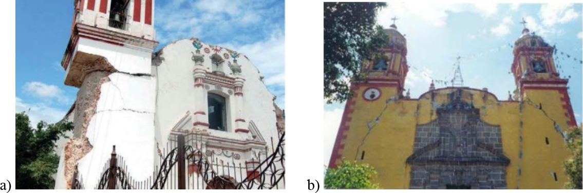
Fig. 1. Trend of deterioration and failure in bell towers attached to adjacent bodies, a) horizontal failure by earthquake with a tendency to tip over at the top by abrupt change in volume. Image taken from of the Ministry of Culture, Government of Mexico (2024), b) diagonal failure by earthquake by abrupt change in section. Image taken from: De la Torre R. O., et. al. (2004).
To understand the structural behavior of this type of towers, it is common to analyze them in isolation, where the modeling of neighboring bodies is avoided in order to carry out simulations quickly. Figures 2 and 3 show the trends of stress concentrations, overturning and deterioration patterns because of seismic inertial forces. Figures 2b and 2c show the modeling of a bell tower in isolation and considering an inverted pendulum type behavior, with fixed base and contact base respectively, where Figure 2b shows a stress concentration with greater magnitude in the abrupt section change with respect to its base, while Figure 2c shows a rigid block type overturning behavior. Figures 2d and 2e illustrate the behavior of the tower considering lateral restraints in the lower part of the tower, simulating the contact with a neighboring body by means of springs, without modeling the complete system with the finite element method. Figure 2e shows a flipping behavior in the change of stiffness. Figures 3c and 3d show the structural deterioration patterns when the towers are modeled as inverted pendulum without lateral restraint and with lateral restraint in the lower zone, respectively.
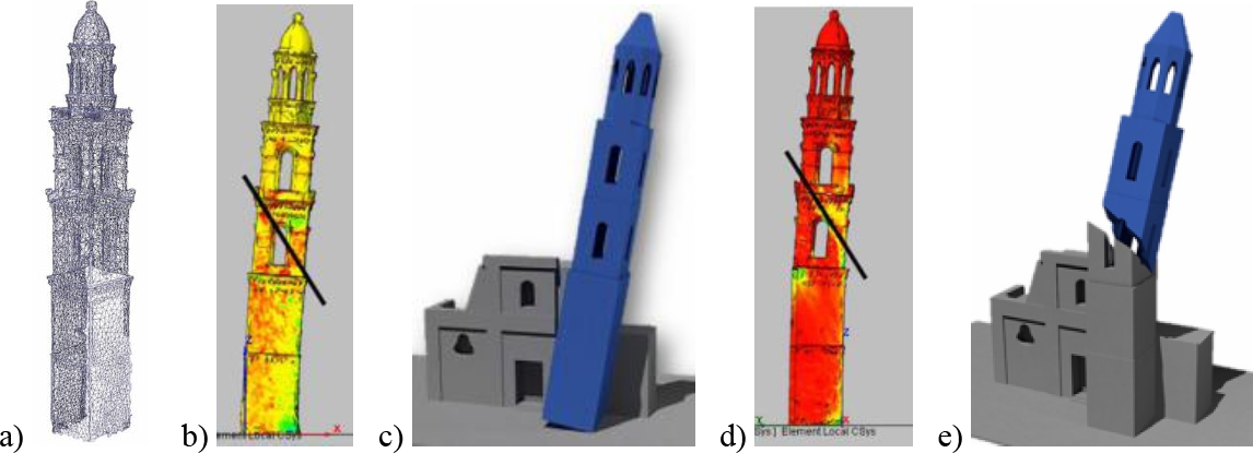
Fig. 2. Stress concentration and overturning trends in bell towers: a) model with finite element (FE), b) stress concentration in isolated tower, c) overturning at the base, d) stress concentration in tower with interaction of adjacent body at the bottom, e) overturning in abrupt section change. Taken from Francesco M., et. al. (2020).
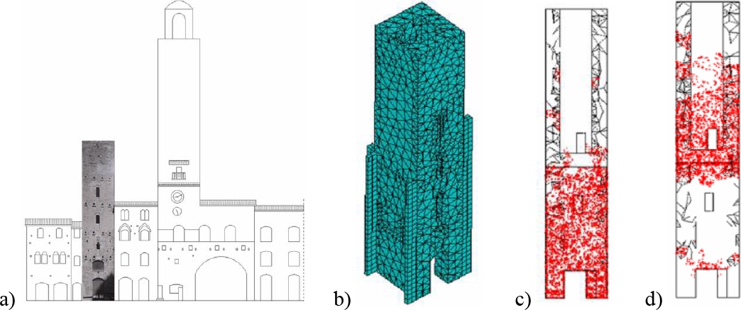
Fig. 3. Patterns of deterioration in bell towers caused by seismic forces: a) front view and interaction of the tower with other adjacent bodies; b) model with isolated FE and lateral constraints; c) cracking zone in isolated tower; d) cracking zone in laterally constrained tower. Taken from: Gianni B., et. al. (2019).
Figure 4 shows the stress concentration trend due to lateral displacements. Figure 4c shows the stress concentration from the intermediate zone towards the top, due to the structural modeling of the isolated tower with restrictions in the lower zone. Figure 4d shows the stress concentration in the lower zone, since there are elements that restrict displacements in that direction; however, the lateral zone in contact with the adjacent body is also not completely decoupled from the adjacent body, which is not observed in the modeling.
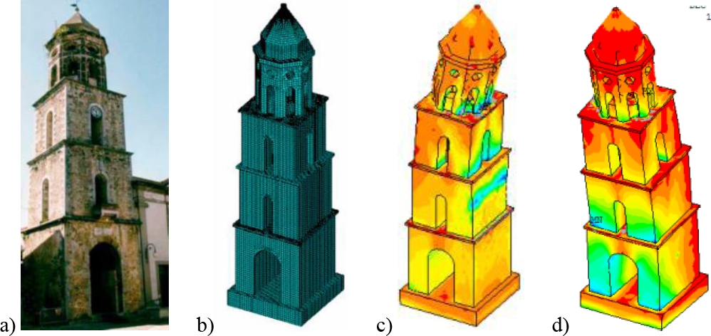
Fig. 4. Trend of stress concentration in bell towers, a) physical bell tower, b) FE model, c) stress concentration in bell tower with lateral restraint at the bottom, d) stress concentration in isolated bell tower. Taken from: Massimiliano F., et. al. (2023).
Figures 5a and 5b show a physical bell tower and its digital FE modeling, while Figure 5c shows the effects of its displacements caused by seismic forces, and Figure 5d plots these displacements with respect to its height to visualize the behavior of the tower.
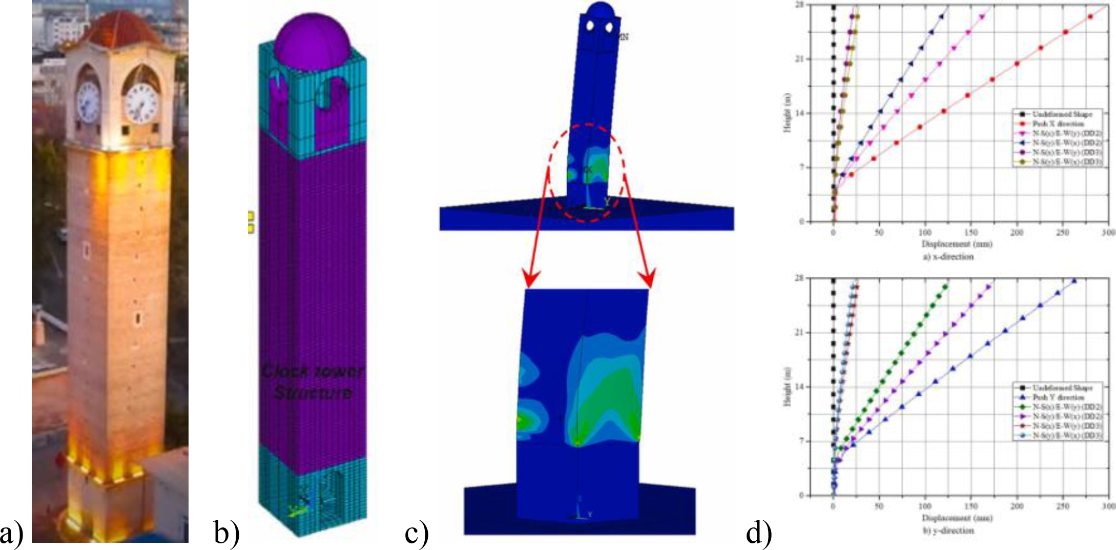
Fig. 5. Displacement trend in bell tower with abrupt section change at the base, a) actual tower, b) FE model, c) concentration of deformations due to lateral displacements, d) displacement graphs in relation to height. Taken from: Hakan E., et. al., (2024).
In Figures 2 to 5, four digital cases are presented; these cases have in common the tendency to present significant lateral displacements as a result of exposure to seismic events; likewise, stress concentrations are observed in the abrupt changes of sections and with the increase in height or at the base when the towers are modeled in isolation. On the other hand, Figure 5 shows that such behavior can be plotted linearly to simulate the trend of displacements and their interaction with adjacent bodies or rigid bases. This type of digital models with FE can be used to simulate the displacement behavior of towers belonging to complete systems of historical buildings or even isolated towers, and to speed up the process it is proposed to use shell type elements. In addition, the ISCARSAH (2003, 2004) principles and guidelines encourage structural studies to be carried out on the complete system and not in isolation.
Figure 6 shows a scale model of a typical temple in Mexico built with irregular historical masonry with lime-sand mortar, as well as its damage patterns simulated on a shaking table (taken from Chávez M., 2010). Once subjected to accelerations at the base, this model presented cracking tendency very similar to that shown in Figure 1, which are historical buildings of irregular masonry joined with lime-sand mortar, under effects left by the 2017 earthquake in Mexico. In the scale model, diagonal cracking patterns are observed in the left tower (Figure 6a), like Figure 1b, while the right tower shows horizontal cracking (Figure 6b), like Figure 1a.
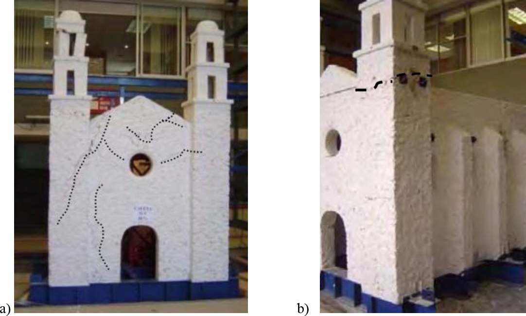
Fig. 6. Main damage to the scale model submitted to seismic actions, a) tendency of deterioration and diagonal cracking in the left tower, b) tendency of horizontal failure in the upper block of the right bell tower. Taken from Chávez M., (2010).
3. SHELL-TYPE FINITE ELEMENT
The finite elements (Figure 7) can be composed of either 3 nodes (u1...u3) giving a triangular shape (C1...C3) having only 5 faces (face 4 is not counted), or it can be composed of 4 nodes (u1...u4) and 6 faces (C1.... C4), these elements have their local axes located in the center of the figure represented by the X, Y and Z axes being represented as E1, E2 and E3 in the figure respectively, they also have their nodes which interact with other finite shell elements as joints to represent a larger element that resembles, in this case, a vault, giving the freedom of modeling using only two types of shell elements. The reason for modeling a triangular or square shell element is mainly for the convergence and rationality of the results obtained, since the nodes show displacements in the 3 axes, being possible to detect such displacements in each node. To visualize the behavior, also the mesh size affects the results, since a fine mesh having many elements consumes more computational resources to obtain results from a single model, so it is a decision of the modeler whether to prioritize the accuracy of the model or the speed of the results. On the other hand, shell elements with rectangular shapes are more implemented in orthogonal, modern and modular buildings, while shell elements with triangular shapes are better suited to irregular and curved shapes, so they are more practical for the modeling of historical temples.
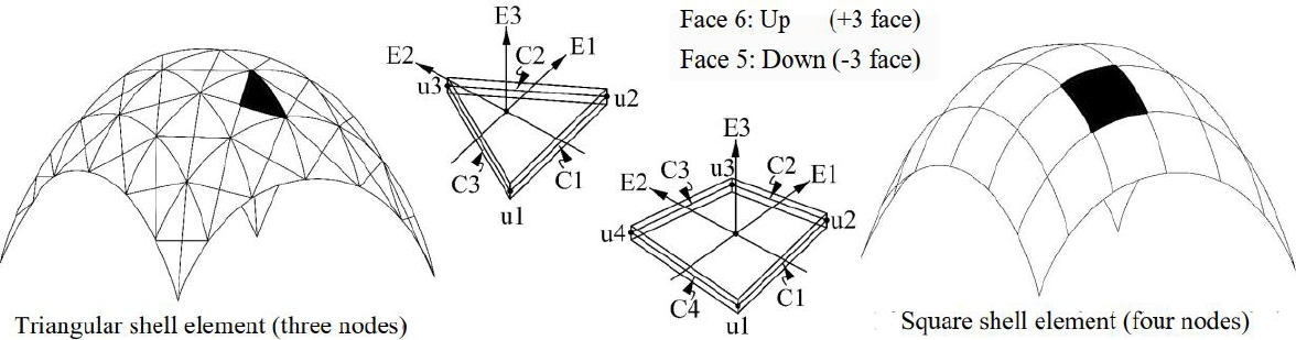
Fig. 7. Vault model based on triangular and square shell FE; representation of axes, faces, and joints. Taken and redrawn from SAP2000v23 (2017), Torres C. A., et. al. (2023).
4. CASE STUDY
The case study is the Temple of the Santa Veracruz, which has a pair of bell towers of approximately 30 m high, made of quarry stone, the main material of this building is irregular masonry, and the walls that make up the structure have a variation of thicknesses reaching thicknesses of 60 cm to 170 cm in various areas of it. Figure 8 shows the architectural elements that make up the structure and their measurements both in elevation and architectural plan. The survey of the temple was taken from the work done by the students of the Specialty in Architectural Restoration of the Section of Postgraduate Studies and Research of the Higher School of Engineering and Architecture, Tecamachalco Unit of the National Polytechnic Institute. This structural geometric survey was carried out by means of tape measures, laser distance meters and plumb bobs.
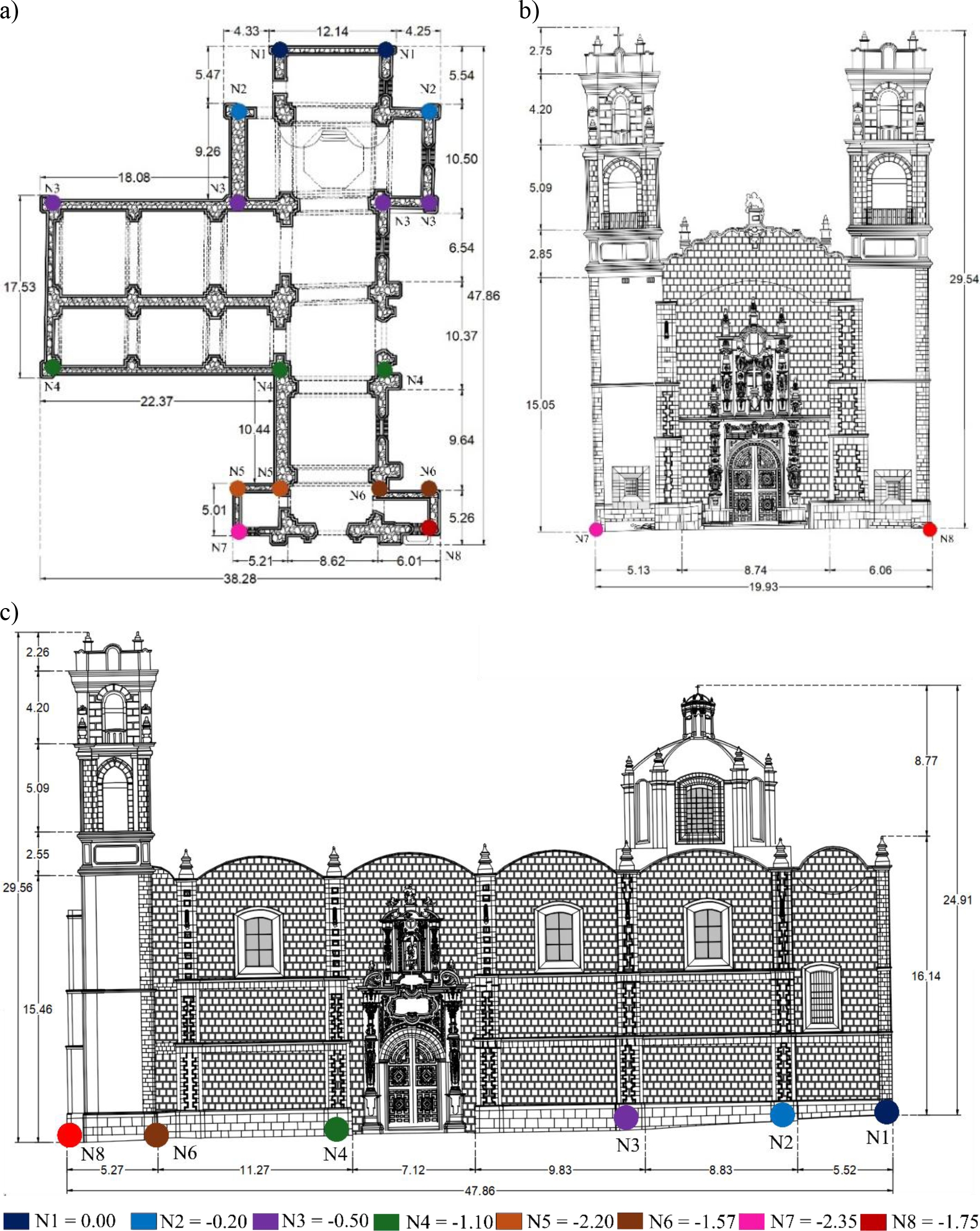
Fig. 8. Temple of Santa Veracruz. a) general architectural plan, b) main facade, c) longitudinal side elevation. Taken and adapted from Zepeda A., et. al. (2014). Where: N = Height level in relation to 0.00. NOTE: all dimensions are meters.
5. DIGITAL STRUCTURAL MODELING
The digital modeling of a historical heritage temple is complex due to the morphology of these buildings, therefore, the methodology implemented for the development of these structures is also complex, since the construction systems that make up each physical-geometric section and the mechanical properties of the materials must be considered. The case study model is developed with shell type finite elements with different thicknesses to represent the building as shown in Figures 9 and 10.
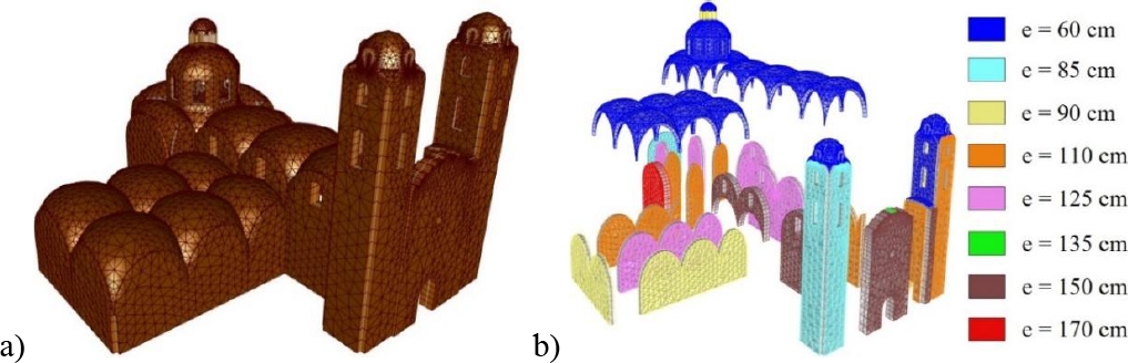
Fig. 9. Models, a) original with FE; b) exploded model of the Temple of the Santa Veracruz made with shell-type FE. Where: e = thickness of the element.
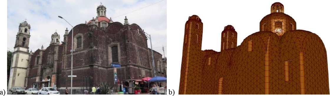
Fig. 10. Photo of the physical building and digital model, a) photo of the Temple of the Santa Veracruz, b) digital model of the Temple of the Santa Veracruz. Image taken from Fernández M. (2024).
The elastic modulus used for structural modeling was 7,063 kg/cm2, Poisson's modulus was 0.17, and the volumetric weight was 1,627 kg/m3 (Torres C., et. al., 2024). Many authors, such as: García N. (2007), Angelillo M. (2014), Chávez M. (2005, 2010), Peña F. et. al. (2010), Meli R., (1998), report and use extremely low tensile stress values ranging from 0.2 kg/cm2 to 3 kg/cm2.
6. DIFFERENTIAL SUBSIDENCE
The subsidence considered for the modeling of the case study has up to -2.35 m difference with respect to the 0.00 m level, causing damage to the structure, these changes are visible in Figure 11 where it can be seen both the physical edition and the digital model with the subsidence applied at its base, the subsidence is also represented in Figure 8 with a color code that shows its magnitude of subsidence from N1= 0. 00 m which is on the right side of Figure 8c, increasing the slope up to N7 and N8 (points with higher subsidence found at the base of the bell towers) which have -2.35 m and -1.75 m differential subsidence with respect to N1. On the other hand, Figure 11a shows the differential subsidence in the physical building in a photograph, while Figure 11b shows the digital model with finite elements which is being subjected to the differential subsidence applying the subsidence from N1 to N8 in a differential way, decreasing the subsidence in relation to the distance of each node, to simulate the behavior of the physical building, the colors of Figure 11b show the behavior of the building in terms of vertical deformations.
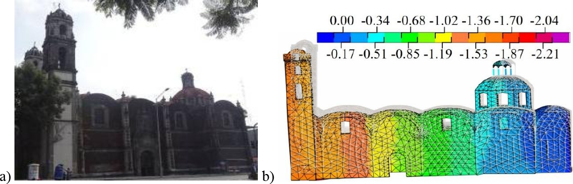
Fig. 11. Differential subsidence, a) actual building, b) digital model of the Temple of the Santa Veracruz created using shell FE. Image taken from Mexico City (2024).
7. SEISMIC ACTIONS
To simulate the seismic effects, accelerograms taken from stations close to the site where the case study is located were used. The accelerograms shown in Figures 12 and 13 correspond to selected seismic signals: Ministry of Communications and Transportation (SCT) B1 and B2 with coordinates 19.394694 LAT N and 94.148678 LONG W, Tlatelolco Campo Libre University Cultural Center (CCUT-CL) with coordinates 19.449858 LAT N and 99.137919 LONG W. Since the accelerograms show the seismic effects of the seismic effects, we used accelerograms taken from stations near the site where the case study is deployed. 137919 LONG W. Since the accelerograms show higher amplitudes in the N90E and N90W directions, these accelerations were considered acting parallel to the short direction of the building, which should be more unfavorable according to the geometric configuration seen in plan of the building. Therefore, in the “X” direction of the model the accelerations N90E and N90W were applied and in the “Y” direction the accelerations N00E and N00W were applied. One of the objectives of this work is to speed up the process of analysis of bell towers that are part of systems, therefore, it was proceeded to look for the periods of time with greater amplitude in the accelerograms and the signals were cut. It was determined 80 seconds of intense phase for each one of them (see figures 14 to 18). Also, to further shorten the analysis times, 12 points with the highest amplitudes in the accelerograms were selected, in which the highest amplitudes (see Figure 19) respected the time steps (∆t) between them, disregarding the acceleration peaks with lower amplitudes.
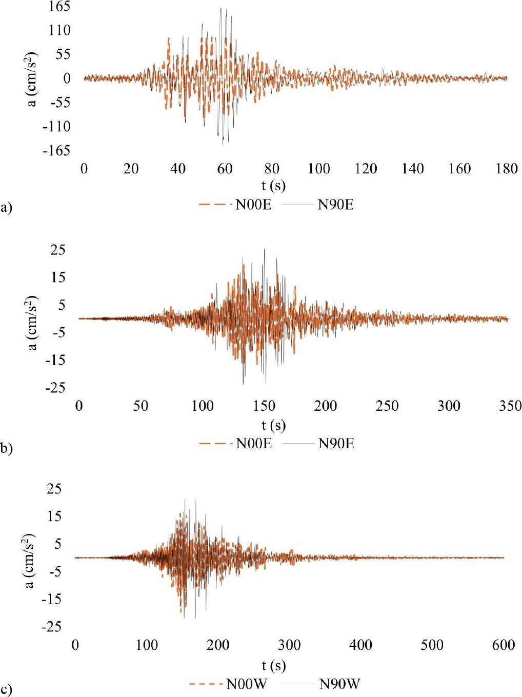
Fig. 12. Complete accelerograms, a) earthquake of 09/19/1985 at station SCT B-1, b) earthquake of 09/09/2017 at station SCT B-2, c) earthquake of 09/09/2017 at station CCUT-CL. Where: t = time (s), a = accelerations (cm/s2). Accelerograms taken and adapted from RAII-UNAM (2014).
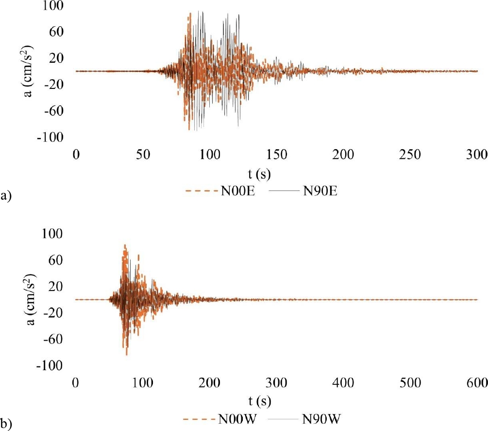
Fig. 13. Complete accelerograms, a) earthquake of 09/19/2017 at station SCT B-2, b) earthquake of 09/19/2017 at station CCUT-CL. Where: t = time (s), a = accelerations (cm/s2). Accelerograms taken and adapted from RAII-UNAM (2014).
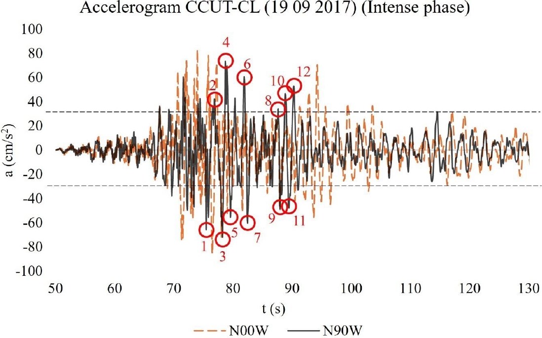
Fig. 14. Accelerogram in intense phase with a duration of 80 seconds of the earthquake of 09/19/2017 at the CCUT-CL station. Where: t = time (s), a = accelerations (cm/s2). Accelerograms taken and adapted from RAII-UNAM (2014).
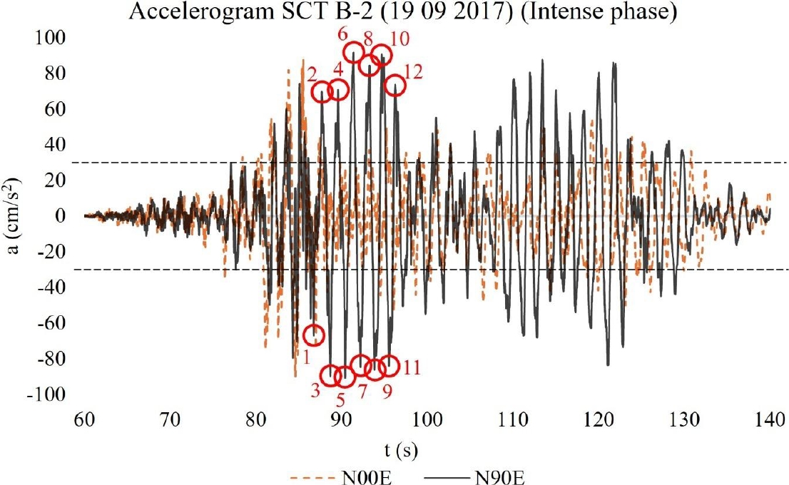
Fig. 15. Accelerogram in intense phase with a duration of 80 seconds of the earthquake of 09/19/2017 at station SCT B-2, where: t = time (s), a = accelerations (cm/s2). Accelerograms taken and adapted from RAII-UNAM (2014).
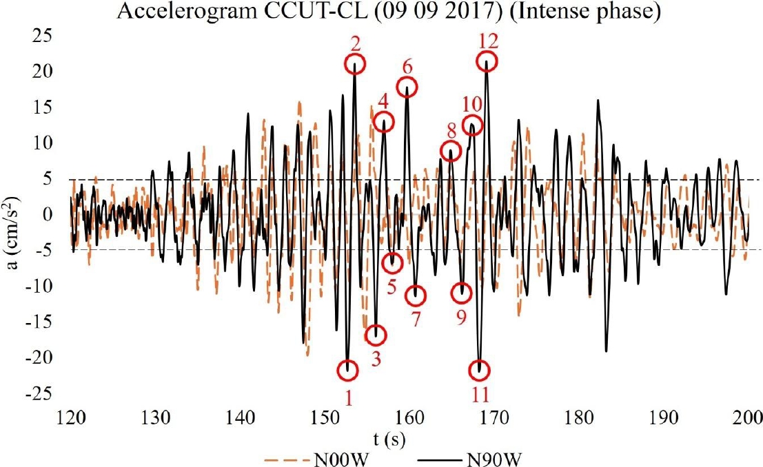
Fig. 16. Accelerogram in intense phase with a duration of 80 seconds of the earthquake of 09/09/2017 at the CCUT-CL station. Where: t = time (s), a = accelerations (cm/s2). Accelerograms taken and adapted from RAII-UNAM (2014).
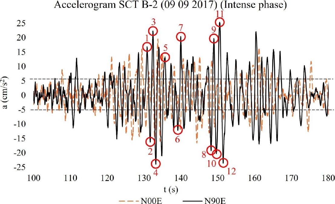
Fig. 17. Accelerogram in intense phase with a duration of 80 seconds of the earthquake of 09/09/2017 at station SCT B-2, where: t = time (s), a = accelerations (cm/s2). Accelerograms taken and adapted from RAII-UNAM (2014).
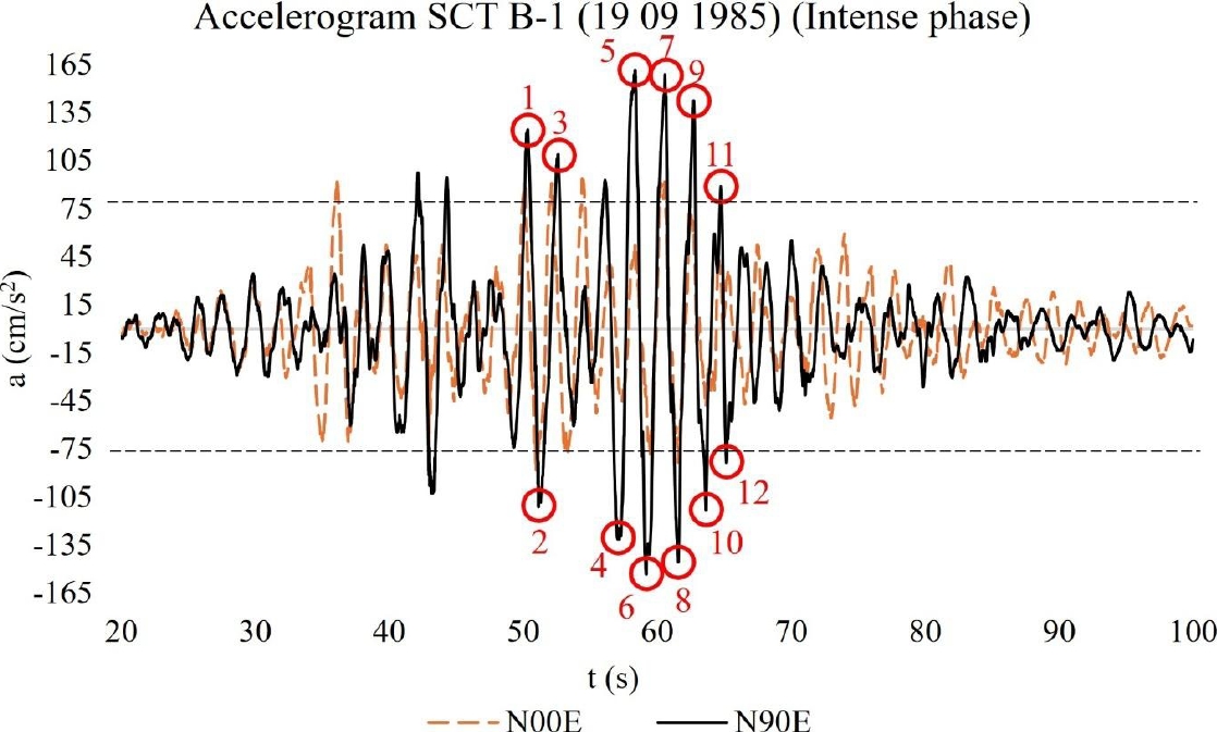
Fig. 18. Accelerogram in intense phase with a duration of 80 seconds of the earthquake of 09/19/1985 in SCT B-1, where: t = time (s), a = accelerations (cm/s2). Accelerograms taken and adapted from RAII-UNAM (2014).
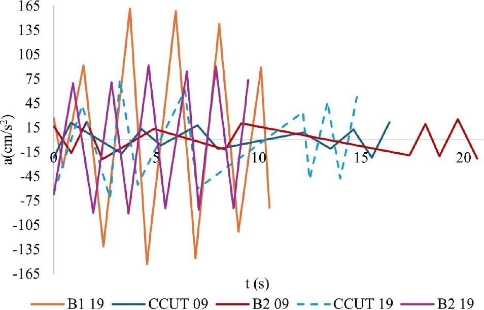
Fig. 19. Accelerograms of 12 Steps Each Time Measured (PCTM) between the selected acceleration peaks of each earthquake. Where: t = time (s), a = accelerations (cm/s2). Accelerograms taken and adapted from RAII-UNAM (2014).
Five earthquakes were determined to make analyses, the first one was detected by station SCT-B1 on 09/19/1985 with magnitude 8.1, the second and third were detected by stations SCT-B2 and CCUT-CL on 09/09/2017 with magnitude 8.2, the fourth and fifth accelerations histories were detected by stations SCT-B2 and CCUT-CL on 09/19/2017 with magnitude 7. It was chosen to implement the four accelerations time histories of the year 2017 (SCT-B2 09, SCT-B2 19, CCUT-CL 09 and CCUT.CL 19) in the analyses, due to the fact that considerable variations were observed in the maximum accelerations between the two dates, being remarkable the fact that the earthquake with magnitude 8.2 (09/09/2017) resulted with lower accelerations than the earthquake with magnitude 7.1 (19/09/2017), being these of 25 cm/s2 and 100 cm/s2 respectively in their highest peaks. Figures 14 to 18 show the thresholds from which the largest accelerations peaks, corresponding to the selection of the 12 steps, were considered, with the purpose of shortening the analysis times.
Currently, access to the building is restricted due to intervention works, and it is guarded by public institutions, which makes its free access and/or temporary instrumentation impossible. In order to validate the seismic analyses using response spectra and accelerograms over time, an inverted pendulum was configured to compare and validate the displacements with respect to an analytical procedure. The inverted pendulum is considered embedded in the base, modeled with shell type finite elements, in which the self-weight of the shaft is neglected, only its stiffness is taken into account, a height of 5 m (h) and a cross section of 50 x 50 cm, with a point load of 30 tons at the top, and an elastic modulus equal to that considered in the irregular masonry of the case study. The pendulum was subjected to the accelerations of Figures 14 to 18. The analytical case (CA) to analyze this pendulum was taken from Torres C. (2023). Figures 20 to 29 show the displacements in this pendulum under actions of accelerograms or complete signal (SC) and intense phase (FI) earthquakes. In addition, alternative signals were proposed, consisting of 12 steps with selected points with t = 1s (12PCS), and 12 steps with selected points with ∆t measured between these points (12PCTM).
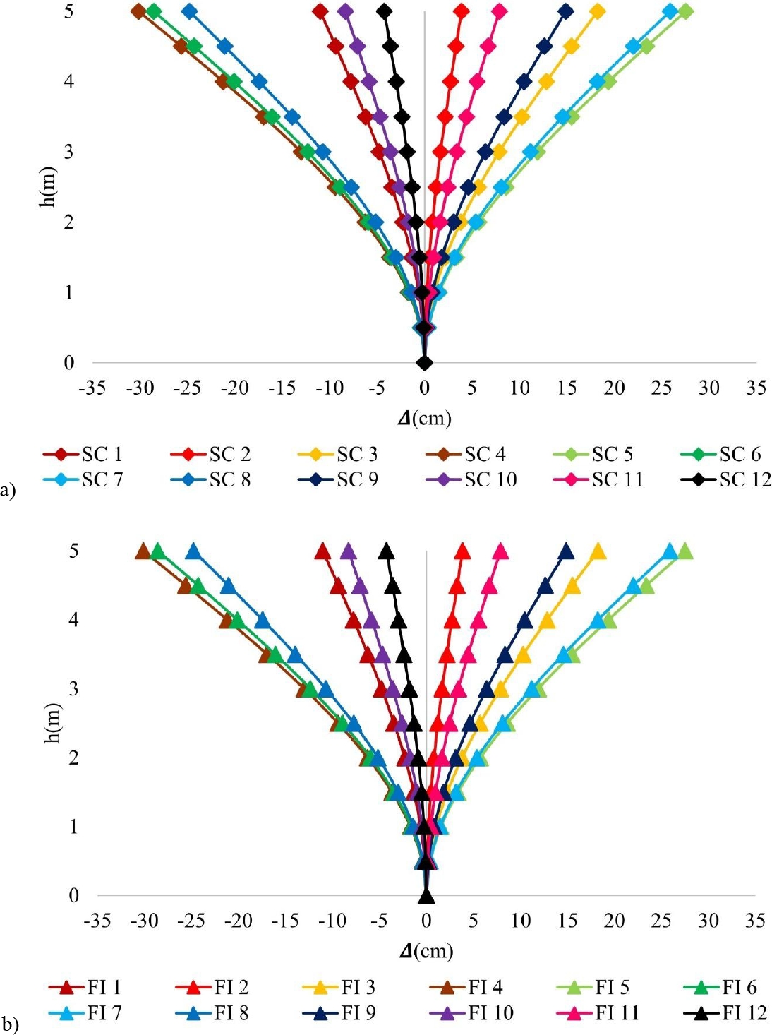
Fig. 20. Inverted pendulum subjected to seismic actions with accelerogram from SCT-B1 (09/19/1985), a) displacements with complete earthquake, b) displacements with intense phase. Where: SC = complete earthquake, FI = intense phase, 𝜟 = displacements.
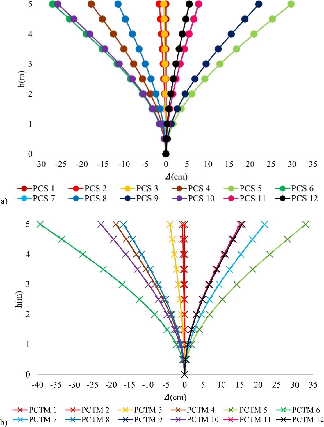
Fig. 21. Inverted pendulum subjected to seismic actions with accelerogram from SCT-B1 (09/19/1985), a) displacements with complete earthquake, b) displacements with intense phase. Where: PCS = steps per second, PCTM = steps per time measured, 𝜟 = displacements.
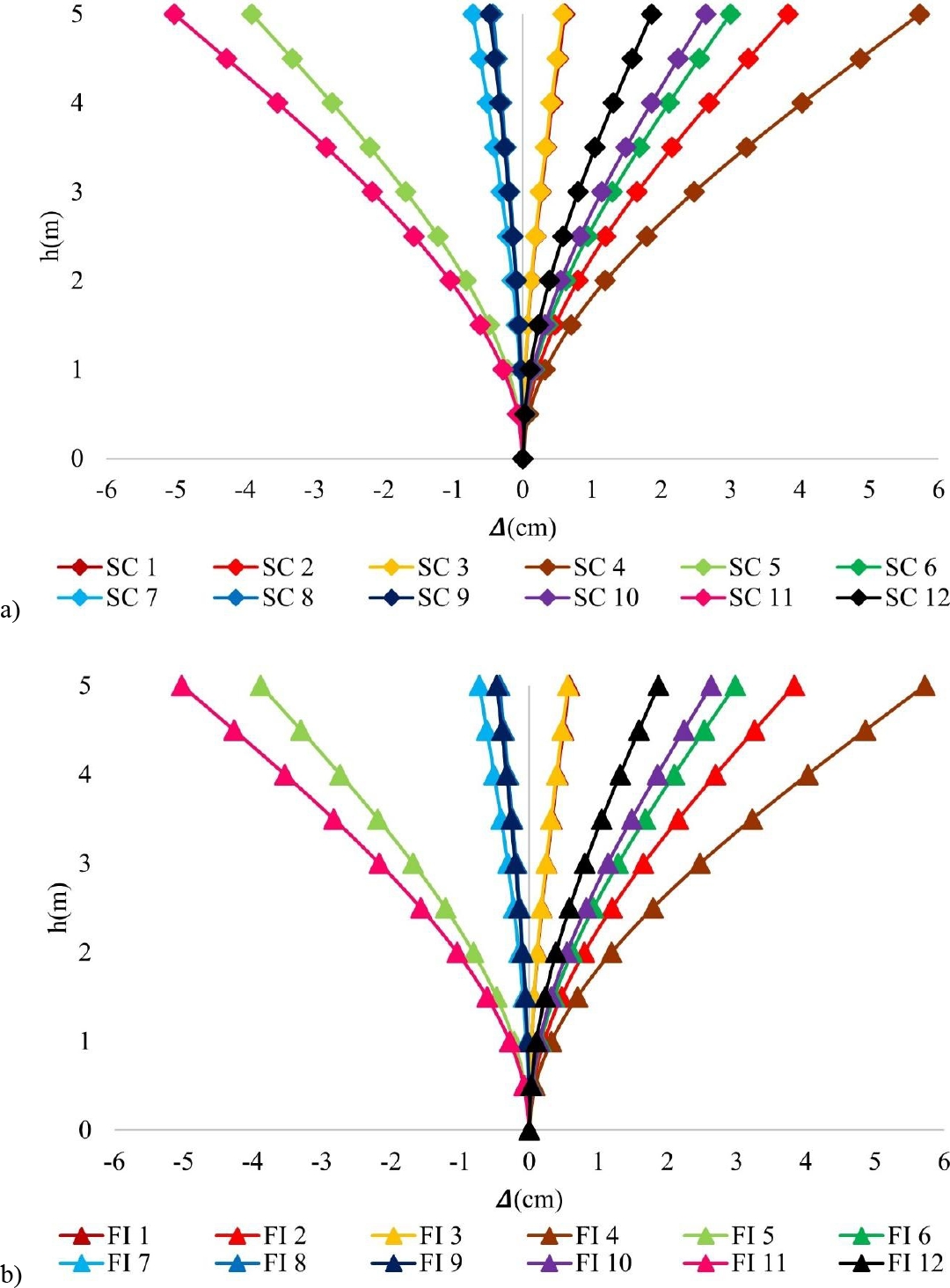
Fig. 22. Inverted pendulum subjected to seismic actions with accelerogram from CCUT-CL (09/09/2017), a) displacements with complete earthquake, b) displacements with intense phase. Where: SC = complete earthquake, FI = intense phase, 𝜟 = displacements.
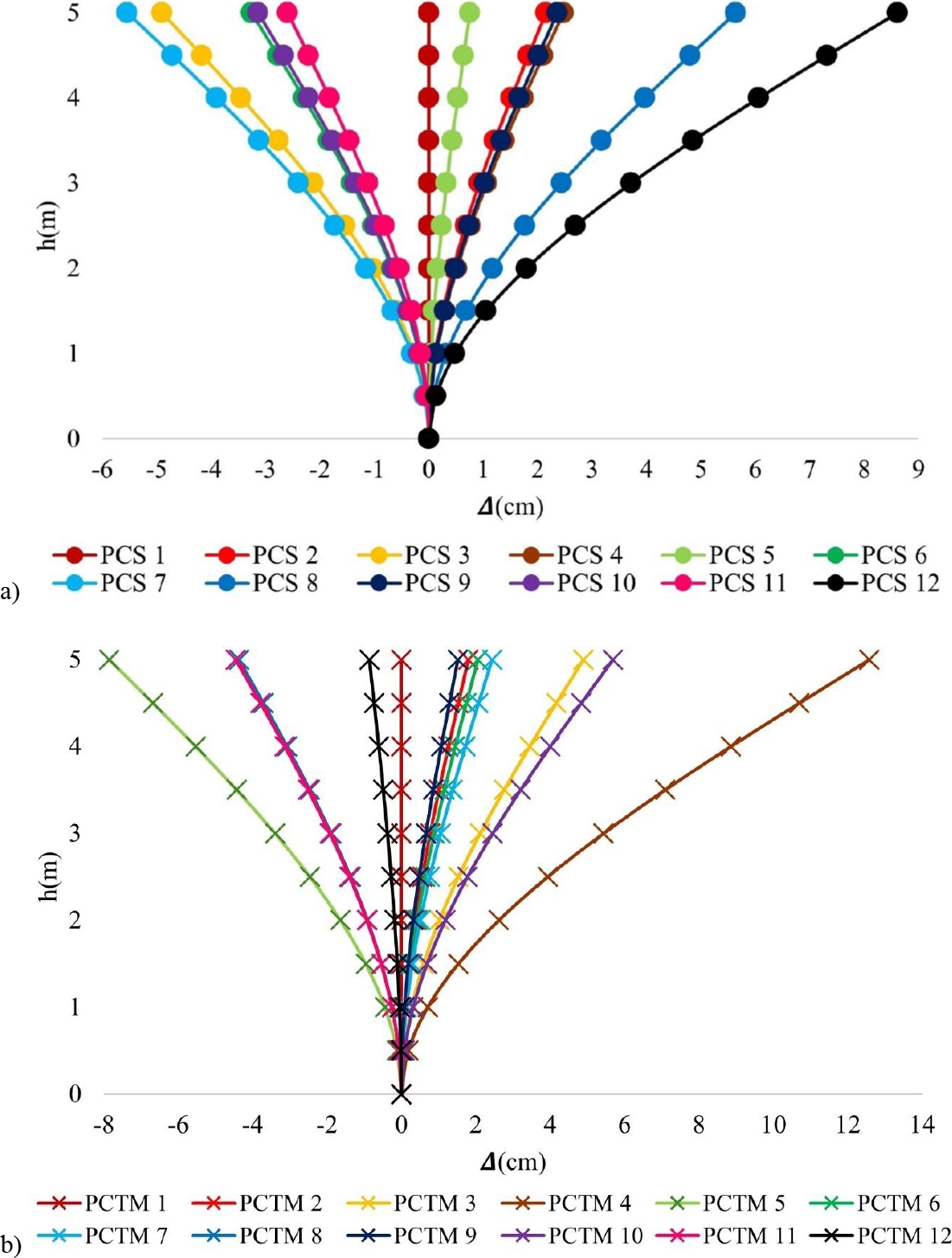
Fig. 23. Inverted pendulum subjected to seismic actions with accelerogram from CCUT-CL (09/09/2017), a) displacements with complete earthquake, b) displacements with intense phase. Where: PCS = steps per second, PCTM = steps per time measured, 𝜟 = displacements.
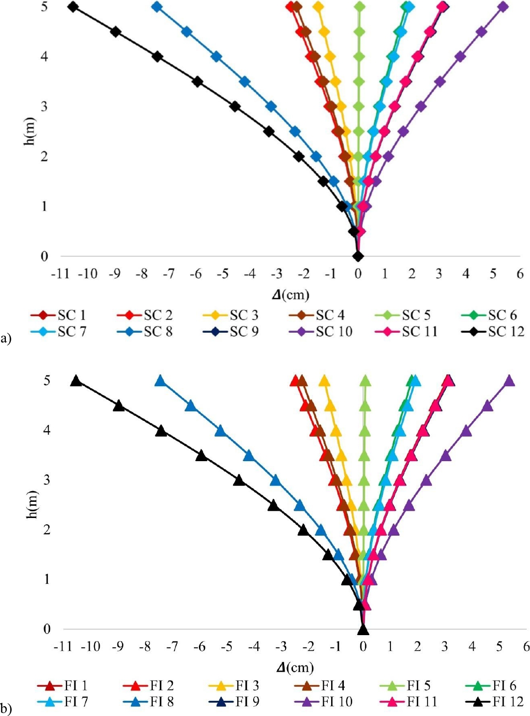
Fig. 24. Inverted pendulum subjected to seismic actions with accelerogram from SCT-B2 (09/09/2017), a) displacements with complete earthquake, b) displacements with intense phase. Where: SC = complete earthquake, FI = intense phase, 𝜟 = displacements.
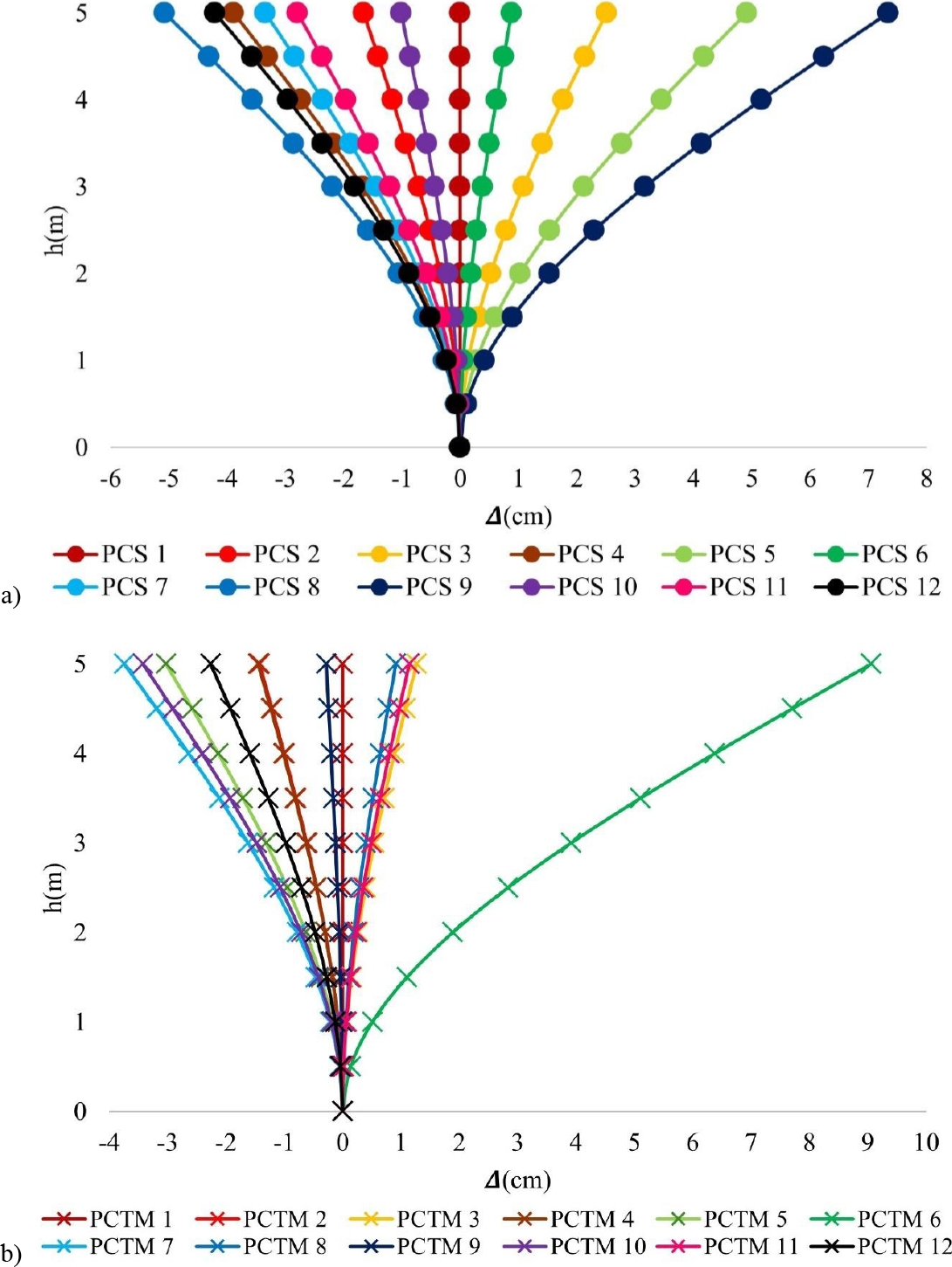
Fig. 25. Inverted pendulum subjected to seismic actions with accelerogram from SCT-B2 (09/09/2017), a) displacements with complete earthquake, b) displacements with intense phase. Where: PCS = steps per second, PCTM = steps per time measured, 𝜟 = displacements.
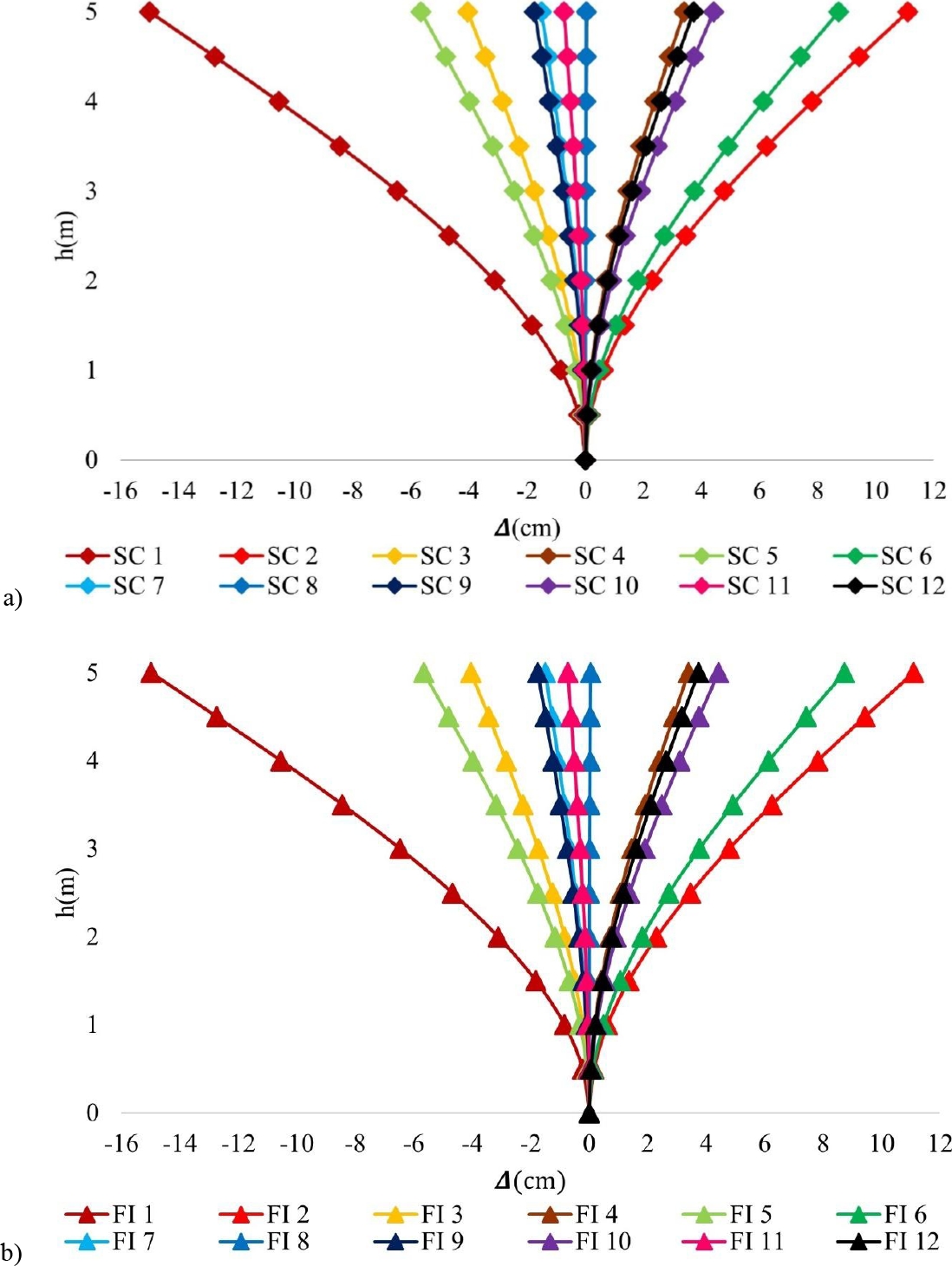
Fig. 26. Inverted pendulum subjected to seismic actions with CCUT-CL accelerogram (09/19/2017), a) displacements with complete earthquake, b) displacements with intense phase. Where: SC = complete earthquake, FI = intense phase, 𝜟 = Displacements.
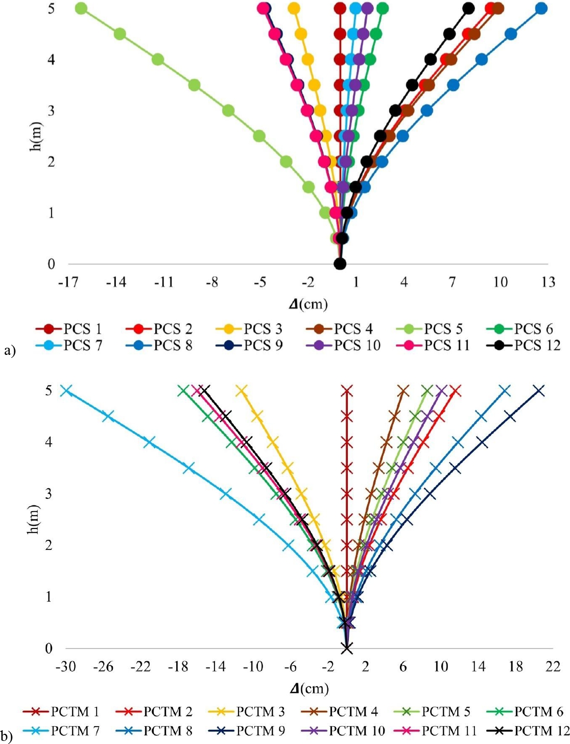
Fig. 27. Inverted pendulum subjected to seismic actions with CCUT-CL accelerogram (09/19/2017), a) displacements with complete earthquake, b) displacements with intense phase. Where: PCS = steps per second, PCTM = steps per time measured, 𝜟 = displacements.
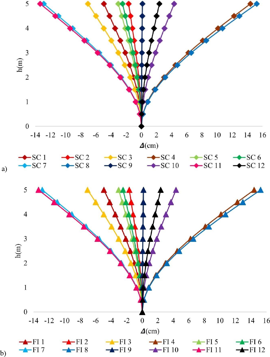
Fig. 28. Inverted pendulum subjected to seismic actions with accelerogram from SCT-B2 (September 19, 2017), a) displacements with complete earthquake, b) displacements with intense phase. Where: SC = complete earthquake, IF = intense phase, 𝜟 = displacements.
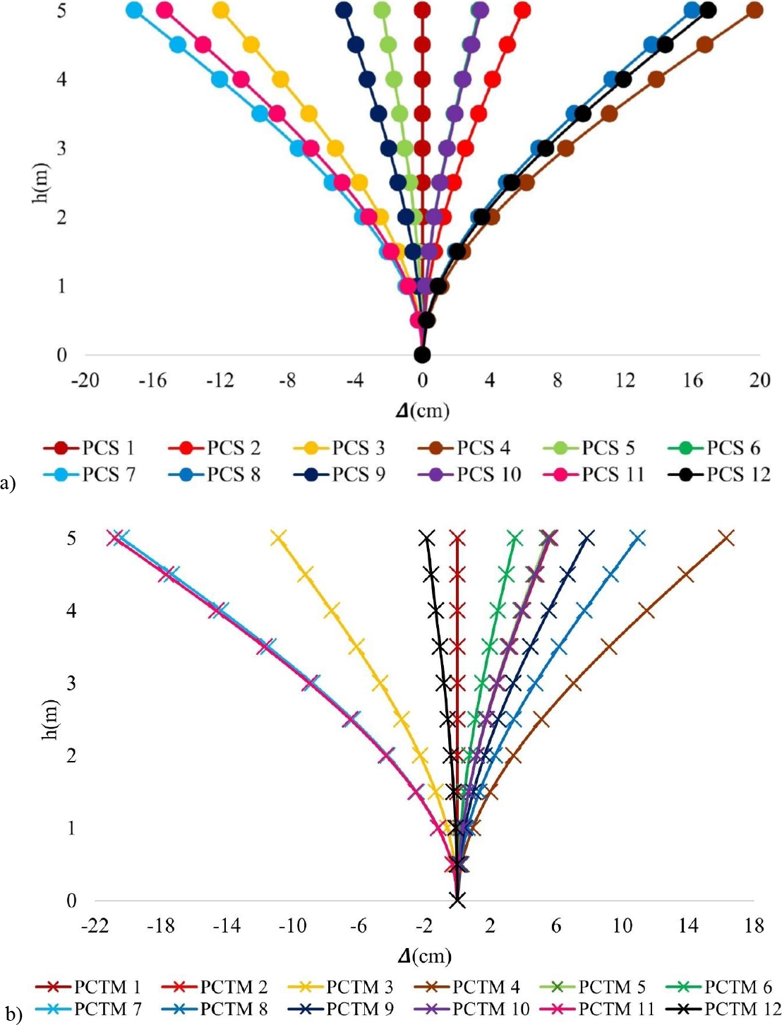
Fig. 29. Inverted pendulum subjected to seismic actions with accelerogram from SCT-B2 (09/19/2017), a) displacements with complete earthquake, b) displacements with intense phase. Where: PCS = steps per second, PCTM = steps per time measured, ?? = displacements.
Figures 20, 22, 24, 26 and 28 show the SC and FI cases in points a and b respectively, in which practically equal displacements are observed, while Figures 21, 23, 25, 27 and 29 show the 12 PCS and 12 PCTM cases in points a and b respectively, these last two cases have a behavior that differs from the first two SC and FI cases. Figures 30 to 34 show the pendulum displacements with each analyzed earthquake, in full time, intense phase and in the time range of the 12 selected points, corresponding to items a, b and c respectively, in addition, in item c the displacements determined with the analytical case (CA) are shown with black points. Based on the results obtained and shown in Figures 20 to 34, it was decided to carry out the analyses only with the FI for the analysis of the complete system.
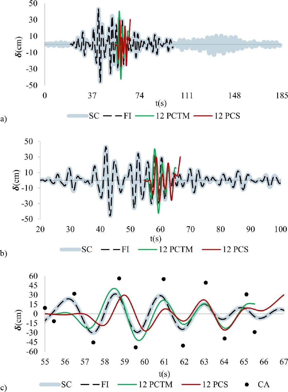
Fig. 30. Superposition of displacements over time, determined with SCT-B1 (09/09/1985), a) SC, FI, 12 PCS, and 12 PCTM over the complete signal time, b) SC, FI, 12 PCS, and 12 PCTM in the intense phase, c) SC, FI, 12 PCS, 12 PCTM, and CA in the time range of the 12 selected points. Where: SC = complete earthquake, FI = intense phase, PCTM = steps per time measured, PCS = steps per second, CA = analytical case.
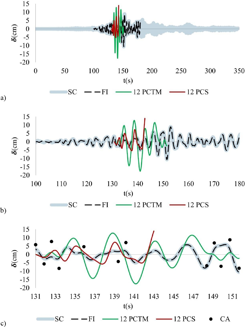
Fig. 31. Superposition of displacements over time determined with SCT-B2 (09/09/2017), a) SC, FI, 12 PCS, and 12 PCTM over the complete signal time, b) SC, FI, 12 PCS, and 12 PCTM in the intense phase, c) SC, FI, 12 PCS, 12 PCTM, and CA in the time range of the 12 selected points. Where: SC = complete earthquake, FI = intense phase, PCTM = steps per time measured, PCS = steps per second, CA = analytical case.
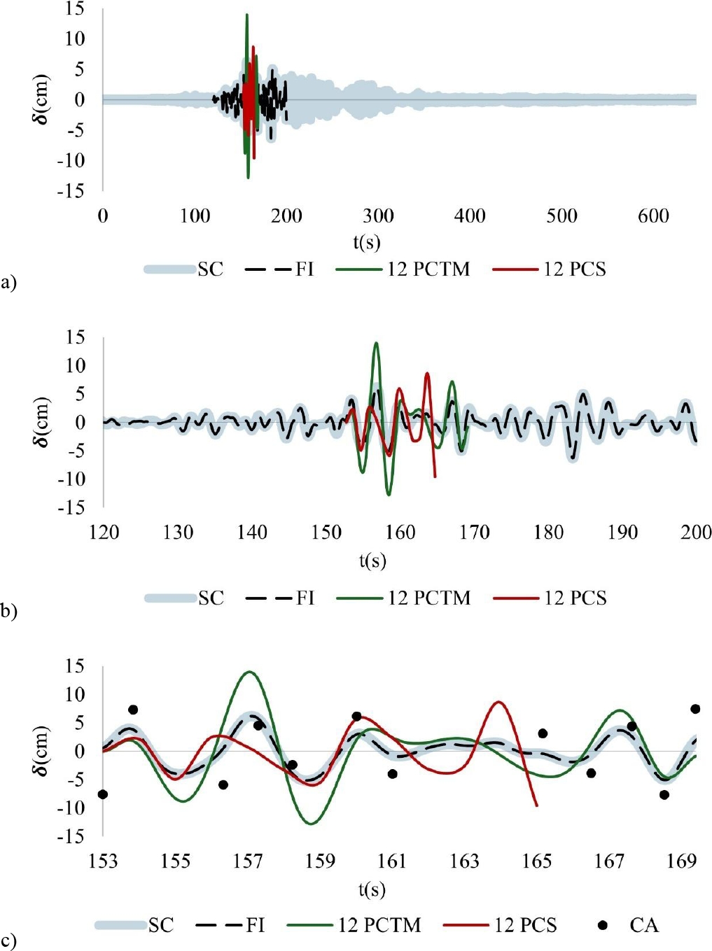
Fig. 32. Superposition of displacements over time, determined with CCUT-CL (09/09/2017), a) SC, FI, 12 PCS, and 12 PCTM over the complete signal time, b) SC, FI, 12 PCS, and 12 PCTM in the intense phase, c) SC, FI, 12 PCS, 12 PCTM, and CA in the time range of the 12 selected points. Where: SC = complete earthquake, FI = intense phase, PCTM = steps per time measured, PCS = steps per second, CA = analytical case.
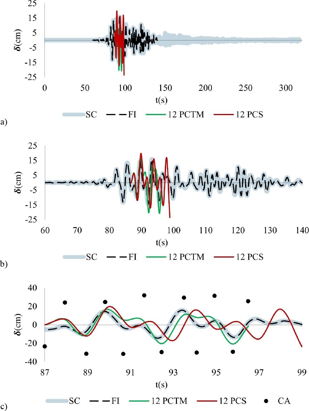
Fig. 33. Superposition of displacements over time, determined with SCT-B2 (19/09/2017), a) SC, FI, 12 PCS, and 12 PCTM over the complete signal time, b) SC, FI, 12 PCS, and 12 PCTM in the intense phase, c) SC, FI, 12 PCS, 12 PCTM, and CA in the time range of the 12 selected points. Where: SC = complete earthquake, FI = intense phase, PCTM = steps per time measured, PCS = steps per second, CA = analytical case.
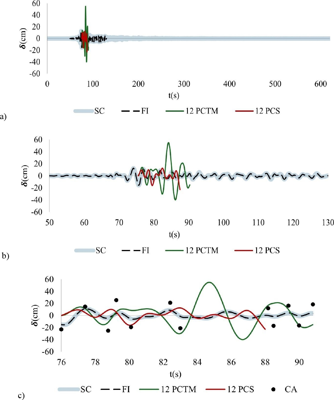
Fig. 34. Superposition of displacements over time, determined with CCUT-CL (19/09/2017), a) SC, FI, 12 PCS, and 12 PCTM over the complete signal time, b) SC, FI, 12 PCS, and 12 PCTM in the intense phase, c) SC, FI, 12 PCS, 12 PCTM, and CA in the time range of the 12 selected points. Where: SC = complete earthquake, FI = intense phase, PCTM = steps per time measured, PCS = steps per second, CA = analytical case.
To compare the displacements and validate them, the site response spectra are presented in Figure 35, these were obtained from SASID (2020), which belongs to the NTCDS-CDMX-2023. The spectra have the following specifications: hyperstability factor k1=0.80, importance factor (group) A1, irregularity factor = 0.7, likewise, the spectra with ductility factors Q=1.0 and Q=1.5 are presented. EPU = uniform hazard spectrum.
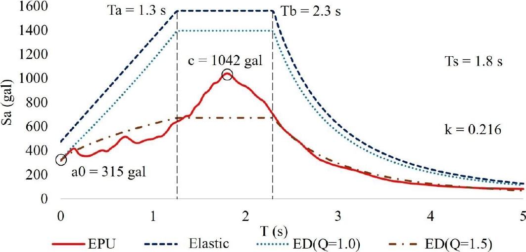
Fig. 35. Response spectra at the site where the building is deployed. Taken and adapted from SASID (2020). Where: Sa = pseudo-acceleration (gal), T = natural period of the structure (s), Ta and Tb = start and end of the plateau, respectively, c = maximum acceleration of the spectrum, Ts = period of the ground, k = ratio between maximum displacements of the ground and the structure, a0 = value of Sa corresponding to T = 0 (maximum acceleration of the ground).
Figure 36 shows the deformations in the previously mentioned pendulum, but now subjected to actions due to response spectra, the different cases can be classified with Q = 1.0, Q = 1.5 (which were affected by Q after obtaining the results) and elastic response spectrum (ERE), each case was analyzed by software of finite elements (S) and by the analytical method (A) to contrast the maximum displacements and angles of rotation that determine the possible overturning of the blocks.
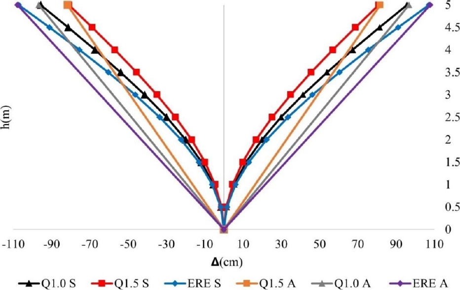
Figure 36. Inverted pendulum subjected to response spectra with ductility Q1.0, Q1.5, and ERE. Where: S = software of FE, A = analytical, ERE = elastic response spectrum.
Figure 37 shows the overturning trend lines of a historical masonry block, where the black line represents the displacements generated in an inverted pendulum type element with continuous finite elements, either linear or quasi-nonlinear, in contrast to the rigid block rotation (represented with the gray line), where 𝜃br is the angle produced at the top of the element as a rigid block, while with the finite element case two different angles are obtained, the first one passing through the flipping failure trend point generating 𝜃f, the second one is generated subsequent to that failure point, generating 𝜃<𝝰, where 𝜃L is the angle measured between the initial block trend and the flip trend from the failure point and 𝜃er is the error angle measured between the flip trend line as rigid block and the flip line trend of the failure block.
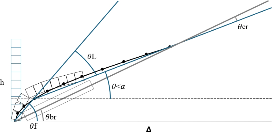
Figure 37. Masonry element subjected to lateral displacement with simulation of tendency to overturn without tensile strength. Where: 𝜃br = angle of rotation as a rigid block, 𝜃f = angle between the horizontal line and the tendency to rotate from the base of the element to the point of tendency to fail by overturning, 𝜃er = angle error measured between the line of tendency to overturn as a rigid block and the tendency of the line of overturning of the failing block, 𝜃L = angle measured between the initial block trend and the overturning trend from the failure point, 𝜃<𝝰 = angle of rotation less than the maximum angle at which overturning occurs, h = height of the element, 𝜟 = lateral displacement.
8. LATERAL DISPLACEMENTS IN THE BELL TOWERS OF THE COMPLETE SYSTEM UNDER COMBINED ACTIONS
For the combinations of seismic actions and subsidence, four cases were considered: C1 = D + Sx + (0.3)Sy, C2 = D + Sy + (0.3)Sx, C3 = D + H + Sx + (0.3)Sy, C4 = D + H + Sy + (0.3)Sx. To measure the displacements, we proceeded to select consecutive nodes on the lateral side at the full height of each of the towers (TI=Left Tower, TD=Right Tower). The displacements were analyzed and plotted in the X and Y directions (Figures 38 to 45), likewise, in the analyses with response spectra, ductility factors Q=1.0 and Q=1.5 with their maximum and minimum displacements were considered. On the other hand, the accelerograms were labeled as: SCT-B1, SCT-B2 09, SCT-B2 19, CCUT-CL 09, CCUT-CL 19 (figures 14 to 18).
The displacements shown in Figures 38 to 45 can be difficult to observe and determine the variations between them, so Table 1 shows the maximum displacements of each combination at the top node (height 29.2m) of each tower, in order to better appreciate the results and see the critical displacements for each case.
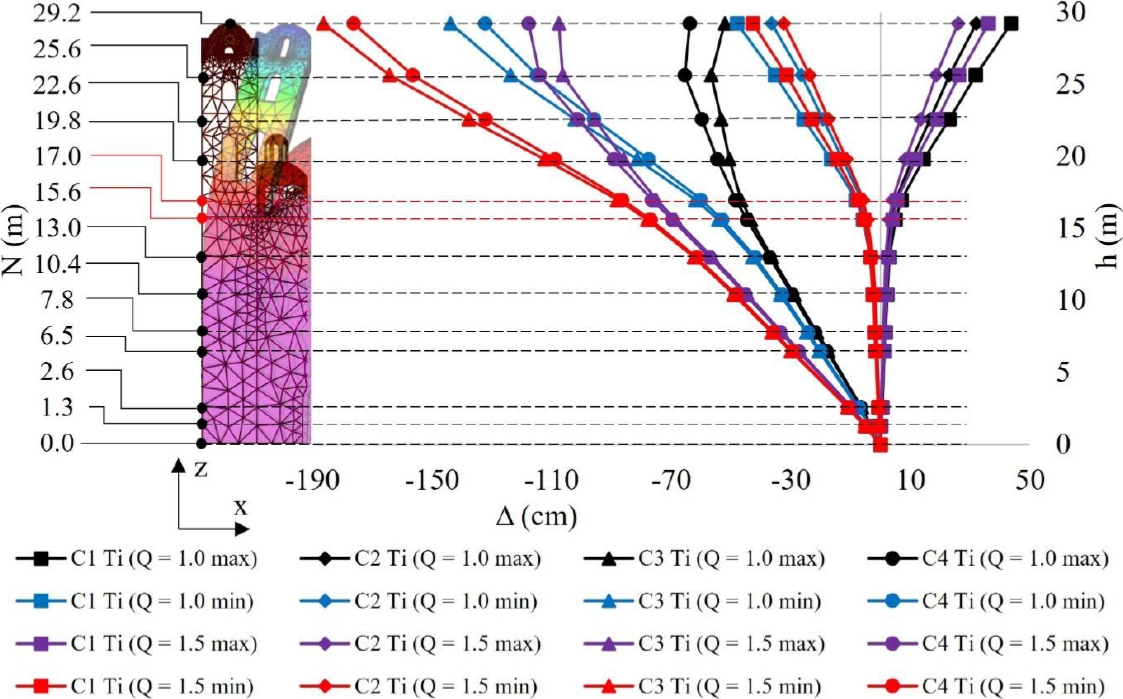
Fig. 38. Displacements in the X direction of the left tower (Ti).
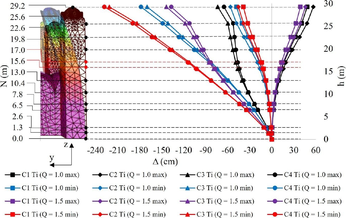
Fig. 39. Displacements in the Y direction of the left tower (Ti).
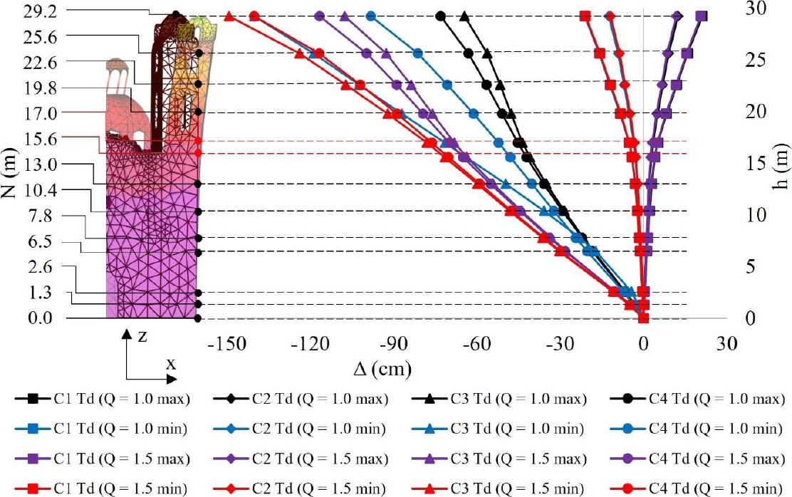
Fig. 40. Displacements in the X direction of the right tower (Td).
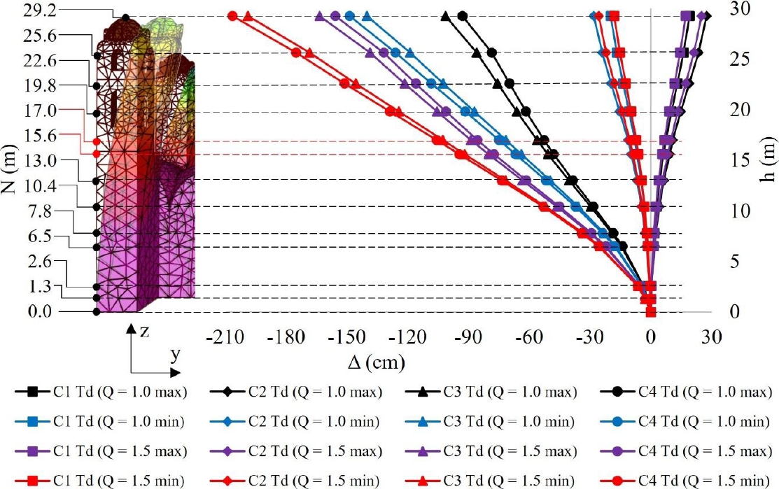
Fig. 41. Displacements in the Y direction of the right tower (Td).
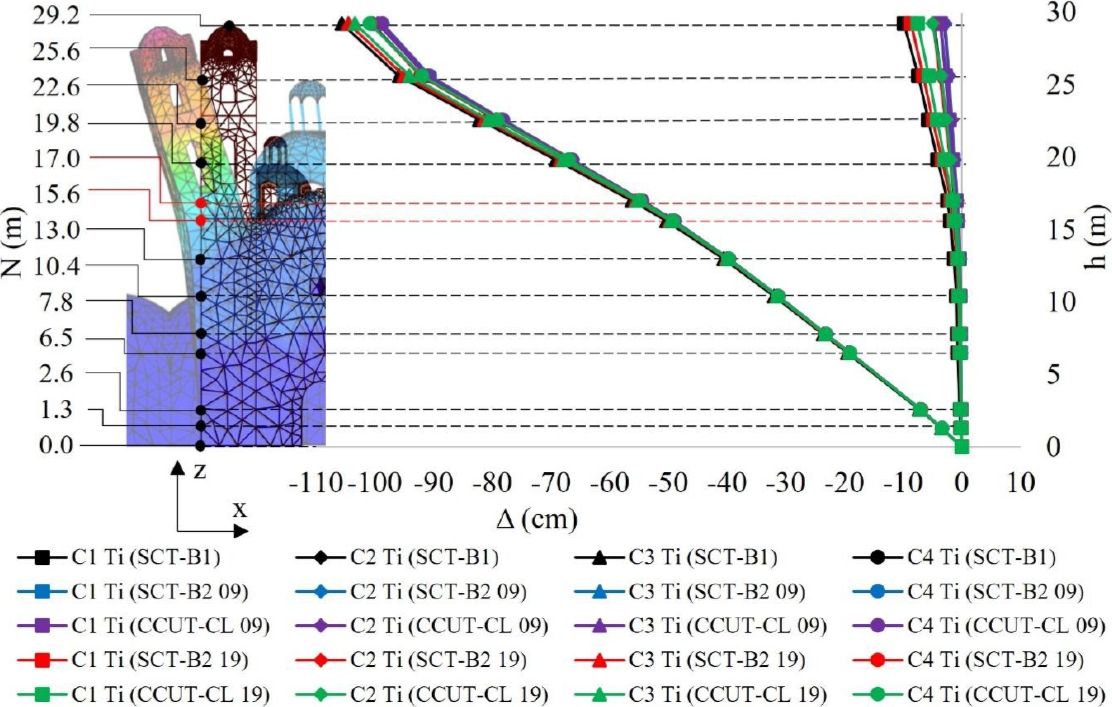
Fig. 42. Displacements in the X direction.
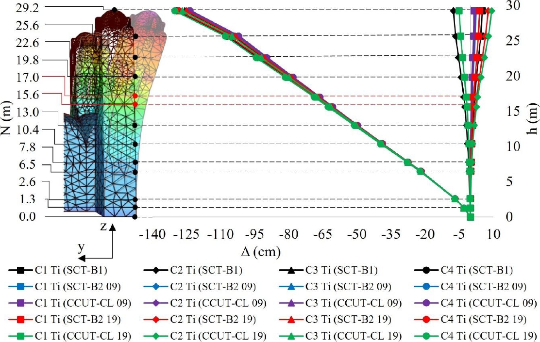
Fig. 43. Displacements in the Y direction.
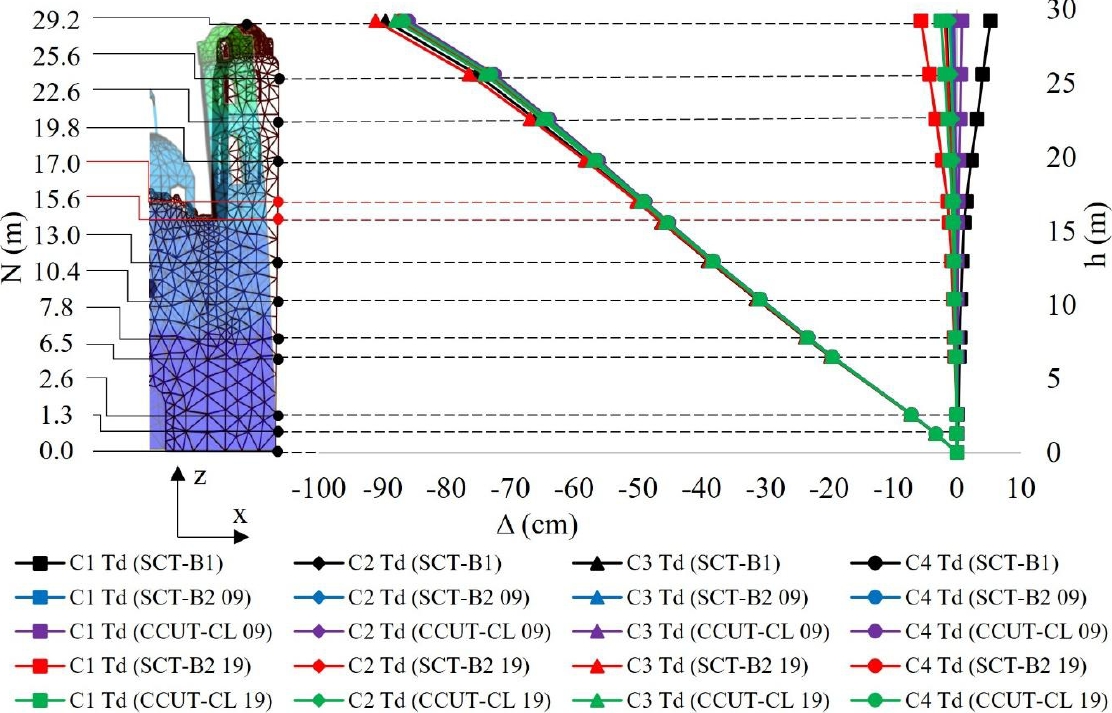
Fig. 44. Displacements in the X direction.
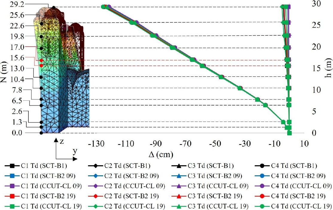
Fig. 45. Displacements in the Y direction.
Table 1. Maximum displacements at the top of bell towers.
| Towers | Acceleration/spectrum | X direction | Y direction | ||||||
| C1 | C2 | C3 | C4 | C1 | C2 | C3 | C4 | ||
| TIA | B1 | -9.80 | -4.71 | -105.65 | -100.56 | 5.15 | -7.50 | -125.76 | -129.27 |
| B2 09 | -3.56 | -2.80 | -99.41 | -98.65 | 1.56 | 2.46 | -122.90 | -123.89 | |
| CCUT 09 | -3.68 | -2.97 | -99.53 | -98.81 | 1.58 | 2.11 | -122.88 | -123.35 | |
| B2 19 | -8.62 | -4.86 | -104.46 | -100.71 | 4.03 | 7.78 | -125.06 | -128.27 | |
| CCUT 19 | -7.53 | -4.99 | -103.38 | -100.83 | -5.02 | 9.27 | -126.79 | -130.14 | |
| TDA | B1 | 5.29 | -1.63 | -89.53 | -87.22 | -3.80 | -3.96 | -124.31 | -124.47 |
| B2 09 | -0.83 | -0.38 | -86.42 | -85.97 | -0.74 | -1.11 | -121.25 | -121.61 | |
| CCUT 09 | 0.85 | -0.37 | -86.37 | -85.95 | -0.67 | -0.99 | -121.17 | -121.49 | |
| B2 19 | -5.54 | -1.83 | -91.13 | -87.41 | -2.50 | -3.48 | -123.00 | -123.98 | |
| CCUT 19 | -2.43 | -1.12 | -88.01 | -86.70 | -2.34 | -5.00 | -122.84 | -125.50 | |
| TIE | Q = 1.0 max | 43.74 | 32.10 | -52.10 | -63.75 | 48.28 | 56.70 | -73.49 | -65.07 |
| Q = 1.0 min | -48.00 | -36.36 | -143.85 | -132.21 | -47.88 | -56.30 | -169.65 | -178.07 | |
| Q = 1.5 max | 36.20 | 25.99 | -107.57 | -117.78 | 39.18 | 45.90 | -143.48 | -136.75 | |
| Q = 1.5 min | -42.59 | -32.38 | -186.36 | -176.15 | -38.57 | -45.30 | -221.22 | -227.95 | |
| TDE | Q = 1.0 max | 21.10 | 12.46 | -64.48 | -73.13 | 19.23 | 27.61 | -101.27 | -92.90 |
| Q = 1.0 min | -21.20 | -12.55 | -140.18 | -98.14 | -19.68 | -28.05 | -140.18 | -148.56 | |
| Q = 1.5 max | 20.68 | 11.70 | -107.70 | -116.67 | 17.32 | 25.06 | -163.44 | -155.69 | |
| Q = 1.5 min | -20.82 | -11.85 | -149.19 | -140.22 | -17.99 | -25.73 | -198.74 | -206.49 | |
It is evident, in Figures 46 to 49, that the maximum displacements in their absolute values do not start at the zero baseline, since some of these start with previous deformations due to subsidence of the base.
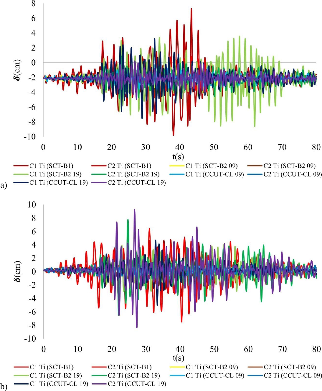
Fig. 46. Superposition of displacements in FI without subsidence, a) X direction, b) Y direction.
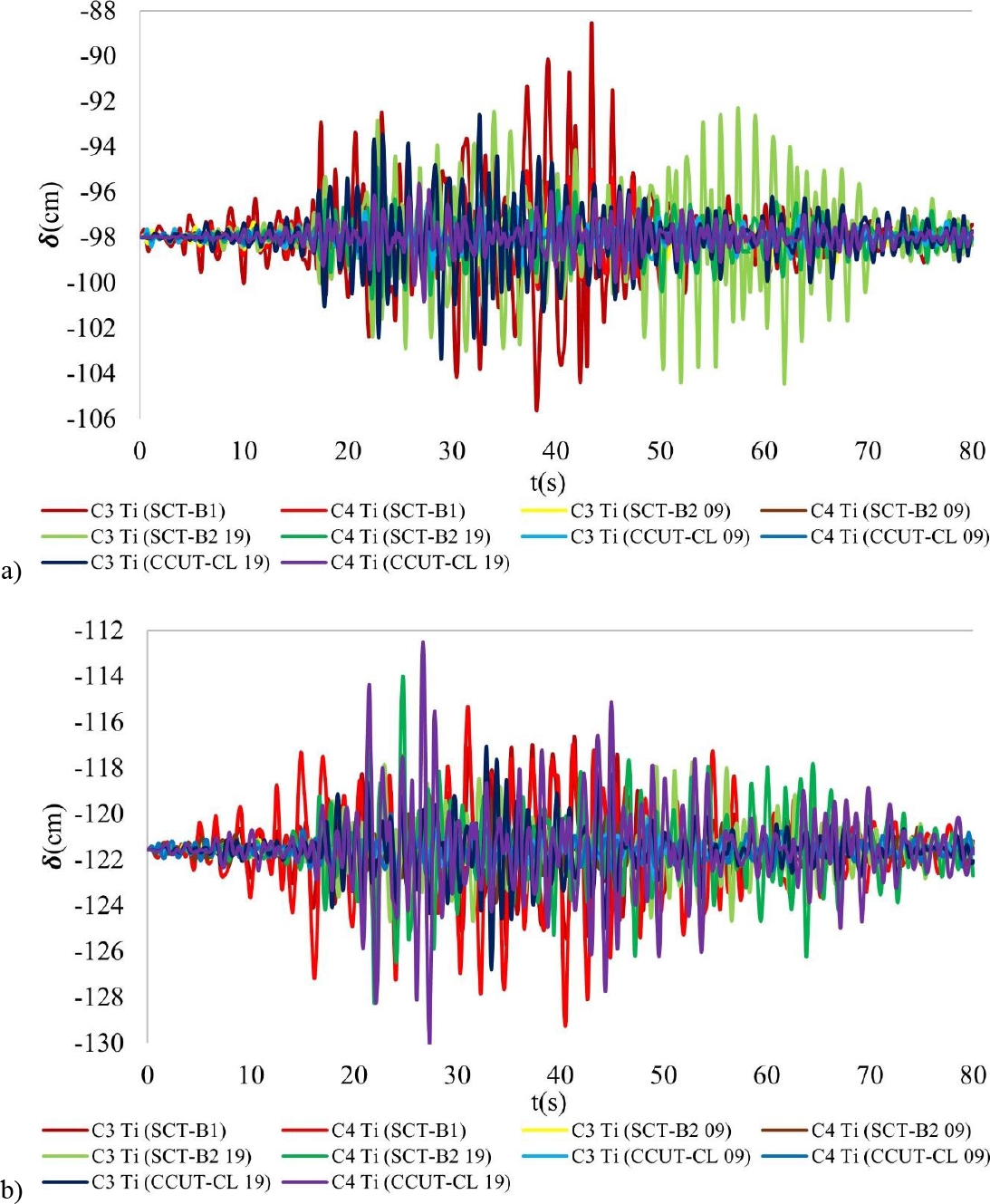
Fig. 47. Superposition of displacements in FI with subsidence, a) X direction, b) Y direction.
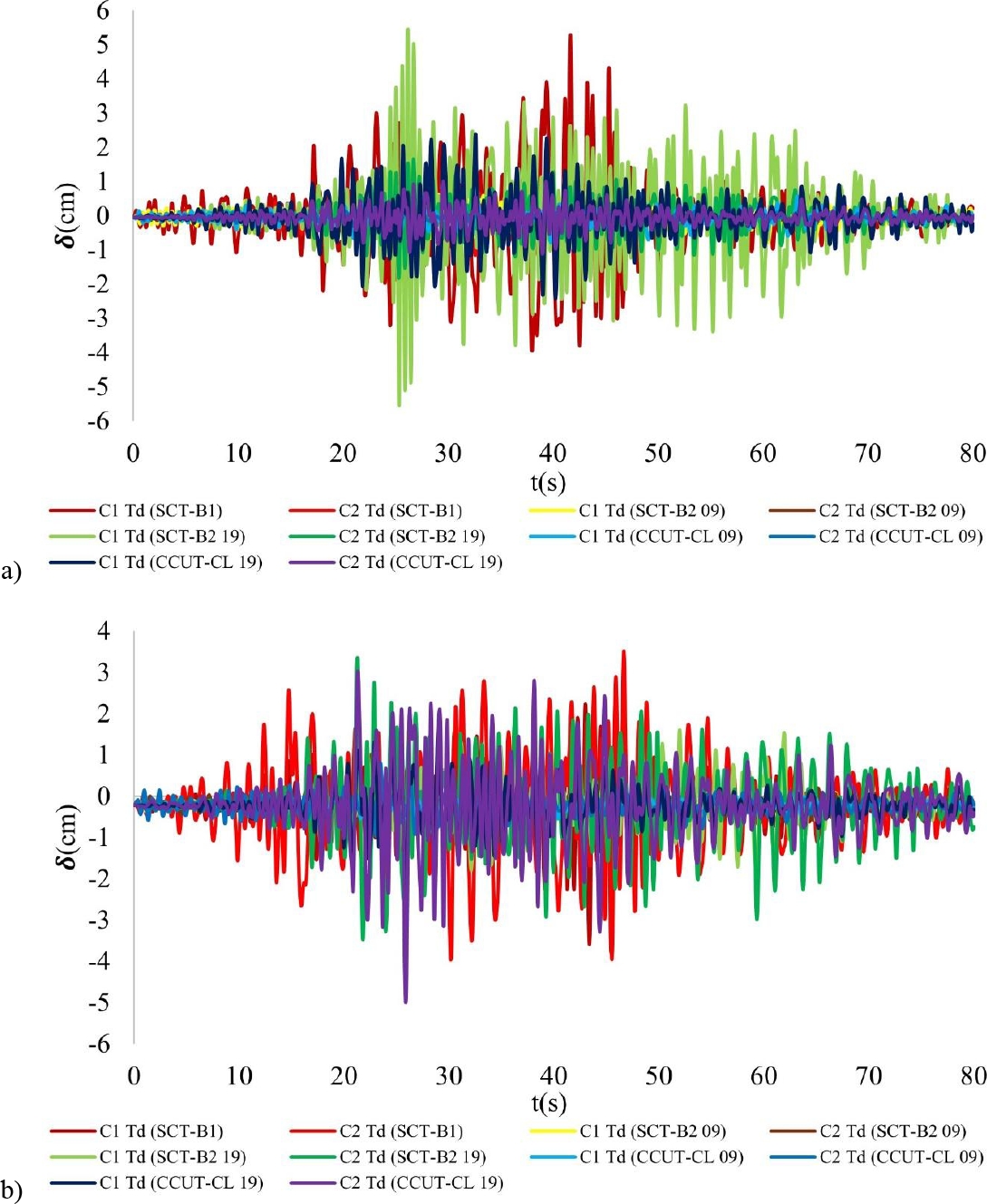
Fig. 48. Superposition of displacements in FI without subsidence, a) X direction, b) Y direction.
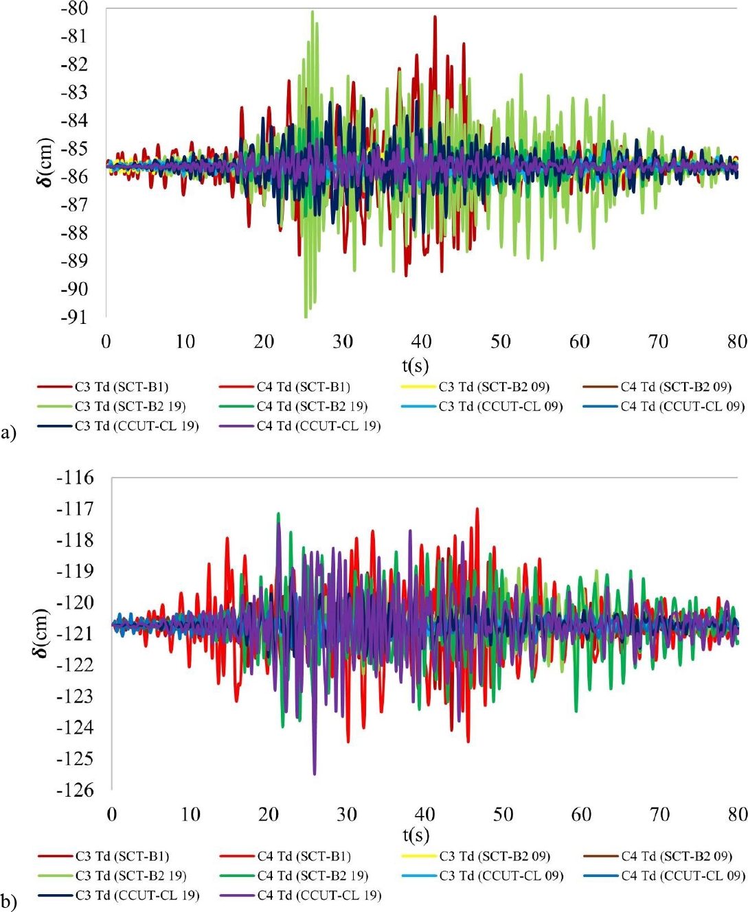
Fig. 49. Superposition of displacements in FI with subsidence, a) X direction, b) Y direction.
Figures 38 to 41 show that some displacement trend lines with spectral seismic actions tend to remain vertical at the top. This is because in some moments of the earthquake the structure is displaced in the opposite direction to the subsidence and tries to verticalize the bell towers when the displacements are positive (in the graphs they are shown as maximums).
9. RATIO OF LATERAL DISPLACEMENTS WITH BLOCK OVERTURNING
According to the premises mentioned by Heyman J. (1969, 1997), Mas-Guindal A.J. (2011) and Huerta S. (2004), regarding the way of working of the masonry used in the construction of historic buildings, it can be considered that the compressive strength is practically infinite, so it is very difficult and almost impossible for historic masonry to fail by crushing, as long as the classical aspect ratios are maintained and the pounding is minimal. For this reason, it can be considered that, when the tensile strength is exceeded, a block begins to detach and twisting mechanisms begin to form, which generates blocks with a tendency to overturn (Figure 50). For this reason, it is feasible to determine the lateral displacements of the bell towers using complete systems by means of FE-based shell models to obtain their rotation angles, subsequently identifying the possible unfavorable blocks and calculating their physical and geometrical properties such as a) dead weight, area and center of gravity. It is important to mention that, as explained by Peña F., (2015), the theory of block overturning also obeys to possible geometric and dynamic asymmetries. Once the displacements were determined with the digital model, the vulnerable blocks to overturning were considered as symmetrical, without loss of material both at the base and in the blocks, the angles of the trend lines of the most unfavorable displacements were measured and the tensile strength was disregarded. Table 2 shows the rotation angles of the most critical cases of Figures 38 to 45 of the vulnerable block at 17 m height with respect to the horizontal line. It is worth mentioning that the angle α is the angle at which the vulnerable block in the bell towers overturns. It is necessary to mention that the values of the angles are absolute and since the block was considered symmetrical, no matter which way it turns, the representation of figure 50 will always be the same, as for the obtained values of the angles, these were measured by drawing turning trend lines according to the direction and inclination of the displacement lines shown in figures 38 to 45. The most unfavorable displacement case was detected in the left tower, in the Y direction, with the case C4 Ti (Q = 1.5 max), which reaches an angle of 5.34°, being the maximum value among all the combination scenarios considered. The critical or limit angle (α) for which the blocks start to overturn is calculated with equation 1 (Figure 50). Expressions 1 to 5 are related to Figure 50.
| (1) |
| (2) |
| (3) |
| (4) |
| (5) |
Where:
W = block density,
α = maximum angle at which overturning occurs,
cg = center of gravity,
cgα = center of gravity of the block at the maximum angle at which overturning occurs,
h = total height of the block,
b = width of the base in the direction of overturning,
bcg = dimension measured from vertex “O” to the vertical line passing through the center of gravity,
hcg = vertical dimension measured from the base to the center of gravity of the block,
θi = i-th angle of overturning at the base,
θri = i-th remaining angle to cause overturning,
cgi = i-th position of the block's center of gravity with rotation at the base with respect to point “O”,
R = distance from point “O” to the center of gravity,
β = angle formed between line “O”-“cg” and the horizontal line of the base,
Γi = i-th angle of the line “O”-“cgi” during overturning,
γ = angle formed between the line “O”-“cg” and the vertical line passing through cg,
xi = i-th horizontal dimension between cgi and “O”.
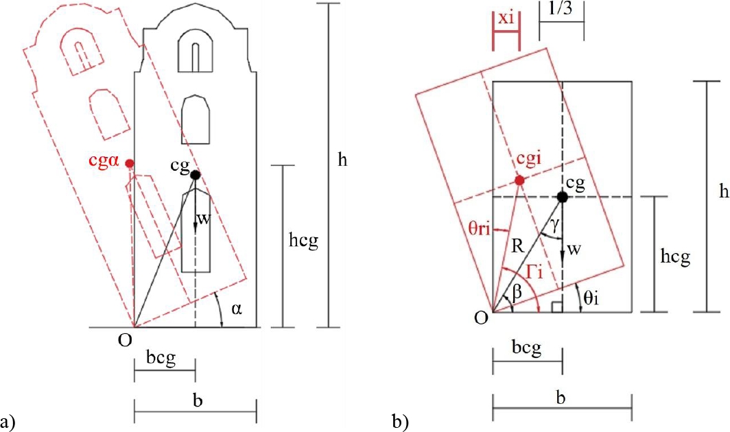
Fig. 50. Rotation of blocks with a tendency to overturn in the towers of the Temple of Santa Veracruz, a) tower block, b) equivalent block. Taken and adapted from Peña F. et al. (2010).
Table 2. Angles of rotation generated by critical displacements in the bell towers of the Temple of the Santa Veracruz.
| Cases | θi° | θri° | xi (m) | θ% | |
| C3 Td (SCT-B2 19) | 1.95 | 19.06 | 9.78 | 1.24 | 9.28 |
| C3 Ti (SCT-B1) | 2.20 | 18.81 | 8.55 | 1.09 | 10.47 |
| C4 Td (CCUT-CL 19) | 3.02 | 18.00 | 5.96 | 0.76 | 14.36 |
| C4 Ti (CCUT-CL 19) | 3.08 | 17.94 | 5.83 | 0.74 | 14.64 |
| C3 Td (Q = 1.5 max) | 3.08 | 17.93 | 5.82 | 0.74 | 14.67 |
| C3 Ti (Q = 1.5 max) | 4.59 | 16.43 | 3.58 | 0.46 | 21.82 |
| C4 Td (Q = 1.5 max) | 4.90 | 16.11 | 3.29 | 0.42 | 23.33 |
| C4 Ti (Q = 1.5 max) | 5.34 | 15.67 | 2.93 | 0.37 | 25.42 |
Figure 51 illustrates the blocks critical to lateral displacements in the bell towers. Figure 51b shows the block that tends to overturn, which is analyzed according to Figures 37 and 50, in addition to considering the values presented in Table 2, where: b = 5.24m, h = 13.63m, w = 284470.37kg.
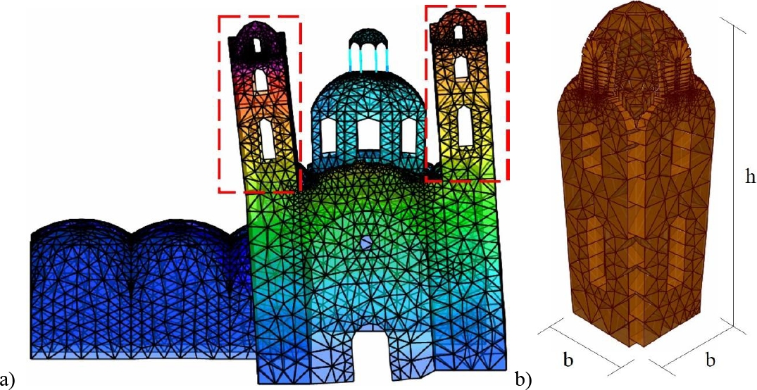
Fig. 51. Critical blocks in bell towers, a) location of critical blocks in the system, b) isolated critical block.
Figure 52 shows the relationship of the horizontal distance from the center of gravity (xi) measured at the vertical edge passing through point “O” of the block with respect to the i-th angle of overturning (θi) of the block. The blue dotted line is the limit of the middle third of safety belonging to the analyzed block, where the centroid moves as the block rotates. Within this range is the black dashed line representing the largest angle that the block reached in the face of seismic actions without subsidence according to Figures 38 to 45, while the green dashed line is the largest angle that was reached (5. 34°) with the combinations including subsidence. Finally, the red dotted line is the angle α at which the block is overturned and xi=0. The angle α resulted in 21.01°.
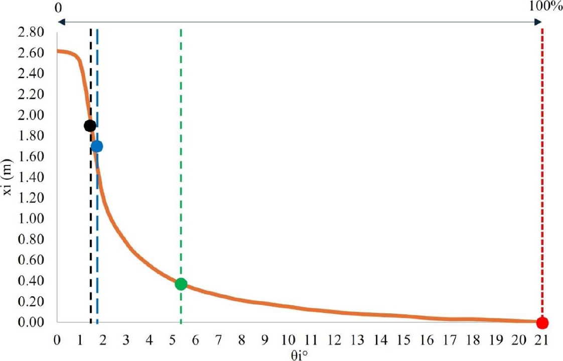
Fig. 52. Relationship between the horizontal distance of the center of gravity (xi) measured at the vertical edge passing through point “O” of the block, and the angle of rotation of the block (θi).
10. DISCUSSION
It is concluded that although there are currently numerical tools to simulate rigid blocks and contact elements for the modeling of historic masonry, these tools consume more computational data and require much more time for their analysis, which is why these tools are currently only used to model relatively small or medium-sized structures and mainly in two dimensions, making them impractical and almost impossible to implement in complete systems in three dimensions. Given that there are many seismic zones around the world, simplified, common, commercial, relatively fast and widely used analysis procedures and tools are required, so that displacements can be checked promptly and efficiently, and thus evaluate the possible risks due to tower overturning. There are many articles that analyze bell towers, however, most of them are modeled in isolation, which contradicts the ISCARSAH-ICOMOS (2003, 2004) principles, where it is mentioned that the analysis should not be performed only in a single part of the buildings, it is necessary to evaluate it completely, so it is not feasible only to safeguard the towers, it is also required to preserve the adjacent bodies. This type of procedures for displacement analysis of the bell towers considering the complete system modeled with FE, allows visualizing the areas susceptible to damage. However, although it is a powerful tool to quickly analyze temples built with historical masonry, it is recommended and also necessary, after having detected these vulnerable areas, to perform structural analysis with specific methods for each of these areas. This article presents the analysis of the complete system, since the isolated analysis would have to take into account the possible vibration contact shaking of the surrounding bodies, since it would be very difficult for the small bodies to collapse first before the towers. For this reason the analysis of the tower separated from the rest of the building is not presented, so it can be concluded that the towers without subsidence would remain within this safety range of the middle third even when subjected to seismic actions.
It was observed that by cutting the signal and using only the intense phase, the displacements were practically the same as when using the complete accelerograms, which meant using only 80 seconds equivalent to 1.2 minutes of each signal, representing the elimination of 87%, 56%, 77%, 73% and 77% of the complete signals (Figures 12 to 18). In this work, the lateral displacements obtained with shell type elements modeled in a complete system subjected to different actions are related to block overturning, rather than analyzing by stresses, since, given the nature of this type of construction systems, they tend to be evaluated with greater certainty under the principles mentioned by some authors such as: Heiman J., (1969, 1997), Mas-Guindal A.J. (2011) and Peña F. (2007). Once the displacements of the structural system are obtained, the angles are determined and the possible overturning of the critical block is checked. For this reason, although environmental vibration (VA) tests are an excellent tool to determine the dynamic properties in buildings, these tools have limitations, since the frequency and amplitude measurement range recorded by most VA accelerometers allow determining dynamic properties in the linear range and with very small displacements, however, for large displacements and/or exceeding the tensile strengths, they no longer have numerical coherence, since this type of buildings tends to separate into macro-blocks. Also, transfer functions are more compatible for analyzing continuous physical systems with small displacements. This is also true for phase angles, coherence functions and cross spectra. This work focused precisely on large displacements and took mechanical properties from the literature, i.e. using parametric methods. To calibrate structural systems it is recommended to carry out VA tests, however, in nonlinear, quasi-nonlinear behavior or with tendency to fracture or overturning of the physical object, such tests are limited and are not compatible to calibrate block rotation and collapse in bell towers, since this type of tests are not valid for large displacements, so that, to calculate bell tower collapses, it becomes more effective to use the rigid block tipping theory, once the lateral displacement tendencies are determined and the rotation angles are obtained. In the analyses carried out with spectral accelerations, displacements of up to 60 cm without subsidence occurred, while in the analyses carried out with time-history accelerations, the maximum displacements did not exceed 10 cm. When taking into account the subsidence at the base, the displacements with spectral accelerations produced a maximum verticality loss of 7.5% with respect to the highest part of the towers, while the time accelerations produced a maximum collapse of 4.5%, which represents a difference of 40% between them.
11. CONCLUSIONS
The behavioral trends of the towers shown in Figures 1 to 6 are similar to the results obtained in the case study of the Templo de la Santa Veracruz, in which it was determined that there is a tendency to suffer greater displacements from the abrupt change of section, this change is located in the upper part of the main nave, which provides lateral support in the lower areas of the bell towers. On the other hand, the use of shell finite elements was adequate for the rapid structural modeling of the temple. Likewise, the responses of the displacements determined with the different accelerograms used for the analyses showed significant differences, where the accelerogram of the complete earthquake (SC) and the intense phase (FI) produced practically equal displacements between them, however, when trying to reduce the analysis times by selecting only 12 specific points with the highest accelerations of these accelerograms, such displacements resulted with greater magnitude than those obtained with SC and FI, even exceeding 200% of the displacements in certain cases, so it is not advisable to use only the maximum accelerations of the accelerograms, since the time history of all accelerations define the response of the system and not only the maximum peaks.
It can also be concluded that, when considering the completely rigid blocks with a tendency to overturning, the results vary in comparison with the elements modeled with finite elements (Figure 37). It is concluded that the overturning failure of the bell towers of the case study has a wide range of safety (Figure 52) in seismic events. However, differential subsidence is a factor that greatly increases the displacements, which position the towers out of their safety third, constantly damaging these elements over time. Particularly for the case study, it is recommended to implement re-leveling measures at the base to avoid future damage. This is why this work is unique, since it combines FE-based tools and rigid block element overturning.
12. ACKNOWLEDGMENTS
Thanks are due to the National Polytechnic Institute (IPN) since part of this text is derived from research projects of the Secretariat for Research and Postgraduate Studies (SIP), for example, from the SIP projects 20181461 and SIP 20195419. We also thank the now SECIHTI (formerly CONAHCYT) for the support provided to the authors.
13. REFERENCES
Angelillo, M. (2014), Mechanics of Mansory Structures. Maurizio Angelillo. Springer. Università di Salerno.
Antonella, S., Carmelo, G., Antonello, R. (2016) “Pre-diagnostic prompt investigation and static monitoring of a historic bell tower”, ELSEVIER, Construction and Buildings Materials, pp 838.
Chávez, M. (2005),Estudio experimental de las propiedades mecánicas de mamposterías de piedra natural. Instituto de ingeniería, UNAM, México.
Chávez, M. (2010), Validación experimental de modelos analíticos para el estudio del comportamiento sísmico de estructuras históricas. Instituto de ingeniería, UNAM. México.
De la Torre, R. O., López, V. R., Salazar, H. A., Roldán, C. J. C. (2004) "Evaluación estructural y comportamiento de las reparaciones efectuadas a edificaciones históricas." Revista de Ingeniería Sísmica, no. 70, pp.1-26. Redalyc, https://www.redalyc.org/articulo.oa?id=61807001
Fernández, M. (2024), “La parroquia de la Santa Veracruz: del esplendor al abandono”, Universidad Nacional Autónoma de México, Revista Electrónica Imágenes del Instituto de Investigaciones Estéticas, última data de acesso ao enlace: 09/08/2024, https://www.revistaimagenes.esteticas.unam.mx/la-parroquia-de-la-santa-veracruz.
Filomena, S., Dimitris, P., Francesca, C., Stefania, S., Francesco, S. (2018), “Experimental and numerical dynamic identification of a historic masonry bell tower accounting for different types of interaction”, ELSEVIER, Soil Dynamic and Earthquake Engineering, pp. 249.
Francesco, M., Alessio, C. (2020), “Structural assessment and seismic of a 14 th century mansory tower”, ELSEVIER, Engineering Failure Analysis, pp. 21.
García, N. (2007), “Funcionamiento y seguridad estructural de los templos conventuales del siglo XVI en México”. Tese doutoral. México; UNAM, México.
Gianni, B., Michele, B., Luciano, G., Giacomo, Z. (2019), “Numerical insights on the seismic risk ok confined masonry towers”, ELSEVIER, Engineering Structures, pp. 725.
Hakan, E., Yusuf, C., Musa, Y. (2024), “Non-linear seismic behavior of historic Adana Great Clock Tower”, ELSEVIER, Structures, pp. 9-12.
Heyman, J. (1969), “Teoría, historia y restauración de estructuras de fábrica”. Inst. Juan de Herrera.
Heyman, J. (1997), “El esqueleto de piedra”. Inst. Juan de Herrera.
ICOMOS, International Council on Monuments and Sites, ISCARSAH, International Scientific Committee on the Analysis and Restoration of Structures of Architectural Heritage (2003), “Carta ICOMOS – Principios para el análisis conservación y restauración de las estructuras del patrimonio arquitectónico”. Editorial Documentation Centre UNESCO-ICOMOS
ICOMOS, ISCARSAH (2004), “Recomendaciones para el análisis, conservación y restauración estructural del patrimonio arquitectónico”. Editorial Documentation Centre UNESCO-ICOMOS
Luca, Z. F., Guiosué, B., Rosario, C., Salvatore, R., Silvia, I., Marica, L. P., Antonino, Q. (2017), “Dynamix investigation on the Mirandola bell tower in post-earthquake”, Springer, Bull Earthquake Eng, pp 316-327.
Mas-Guindal, A. J. (2011), “Mecánica de las estructuras antiguas o cuando las estructuras no se calculaban”. Munillaleria.
Massimiliano, F., Angelo, L., Donato, A., Alberto, M., Alberto, M. A. (2023), “Seismic vulnerability analysis and structural rehabilitation of a historical masonry tower”, ELSEVIER, Procedia Structural Integrity, pp 1096.
Meli, R. (1998), “Ingeniería estructural de los edificios históricos”, ICA, México.
MexicoCity (2024), “Santa Veracruz”, Gobierno de la Ciudad de México, Turismo de colores, Fotografía de Jonathan Cardy, última data de acesso ao enlace: 09/08/2024, https://mexicocity.cdmx.gob.mx/venues/santa-veracruz-church/?lang=es
Peña, F. (2007), “On the dynamics of rocking motion of single rigid-block structures”, Earthquake Engineering and Structural dynamics, 2007; 36:2383-2399, Wiley InterScience (https://www.interscience.wiley.com). DOI: https://doi.org/10.1002/eqe.739
Peña, F., Meza, M. (2010), “Seismic assessment of bell towers of Mexican Colonial churches”, Adv. Mater. Res. 133 585–590.
Peña, F. (2015), “Modelo simplificado para el estudio del balanceo asimétrico de cuerpos rígidos esbeltos”
RAII-UNAM (2014), “Red Acelero grafica del instituto de Ingeniera de la UNAM”. Los datos sísmicos fueron proporcionados por la Red Acelerográfica del Instituto de Ingeniería (RAII-UNAM), producto de las labores de instrumentación y procesamiento de la Unidad de Instrumentación Sísmica. Los datos son distribuidos a través del Sistema de Base de Datos Acelerográficos en web: http://aplicaciones.iingen.unam.mx/AcelerogramasRSM/.
SAP2000v23 (2017), “CSI Structural Analysis and Design”. Editorial Computers & Structures, Inc., pp. 204.
SASID (2020), “Aplicación Normas Técnicas Complementarias para Diseño por Sismo de la Ciudad de México (NTCDS-CDMX-2020)”, Fecha de generación de los espectros: 17/05/2024, última fecha de acceso al enlace: 05/08/2024, https://sasid.unam.mx/SASIDV1/default.aspx.
Secretaría de Cultura, Gobierno de México (2024), “Guía para la conservación de bienes culturales, Monumentos históricos y artísticos”, CULTURA, INAH, pp 4.
Torres, C. A., Ruiz, C. (2023), “Tácticas de modelación estructural con elementos tipo shell en inmuebles históricos de mampostería irregular”, Memorias 4CIHCLB, IV Congreso Internacional, pp. 1-12.
Torres, C. (2023), “Análisis lineal y no-lineal de estructuras históricas de mampostería irregular, comparación entre elementos sólidos y shell”, Memorias 4CIHCLB, IV Congreso Internacional, p. 2.
Torres, C. A. (2023), “Procedimiento sistémico y propiedades de la mampostería irregular para el análisis estructural de edificios históricos”, Editorial Restauro Compas y Canto, ISBN digital: 978-607-99572-4-7, pp. 72-88.
Torres, C., Rosas, J., Pérez, O. (2024), “Numerical-vector succession for the graphic structural analysis of masonry historic buildings with arches and symmetrical systems”, Revista ALCONPAT, 14 (2), pp. 191 – 210, DOI: https://doi.org/10.21041/ra.v14i2.717
Zepeda, A., Montero, J. A., Benítez, S. I. (2014), “Inmuebles históricos, Plantas y Cortes Arquitectónicos de la Iglesia Santa Veracruz”, IPN, ESIA Tecamachalco, Seminario de Titulación.