![]()
| Basic Research | https://doi.org/10.21041/ra.v14i2.717 |
Numerical-vector succession for the graphic structural analysis of masonry historic buildings with arches and symmetrical systems
Sucesión numérico-vectorial para el análisis estructural gráfico de edificios históricos de mampostería con arcos y sistemas simétricos
Sequência vetorial-numérica para a análise estrutural gráfica de edifícios históricos de alvenaria com arcos e sistemas simétricos
C. Torres1* , J. Rosas2, O. Pérez2
1 Research professor at Sección de Estudios de Posgrado e Investigación (SEPI), Escuela Superior de Ingeniería y Arquitectura Unidad Tecamachalco (ESIA UT), Instituto Politécnico Nacional (IPN), 53950, Naucalpan de Juárez, Estado de México, México, http://www.sepi.esiatec.ipn.mx.
2 Bachelor´s student at Escuela Superior de Ingeniería y Arquitectura Unidad Tecamachalco (ESIA UT), Instituto Politécnico Nacional (IPN), 53950, Naucalpan de Juárez, Estado de México, México, http://www.sepi.esiatec.ipn.mx.
*Contact author: ktcate2@hotmail.com; ctorresmo@ipn.mx
Received: 22/12/2023
Revised: 10/05/2024
Accepted: 14/05/2024
Published: 15/05/2024
| Cite as: Torres, C., Rosas, J., Pérez, O. (2024), “Numerical-vector succession for the graphic structural analysis of masonry historic buildings with arches and symmetrical systems”, Revista ALCONPAT, 14 (2), pp. 191 - 210, DOI: https://doi.org/10.21041/ra.v14i2.717 |
ABSTRACT
The objective of this research is to denote the application of numerical-vector succession in the structural analysis of historical masonry buildings, with arches and symmetrical systems, including mathematical processes in ancient graphic analysis, emphasizing the importance of loads in the structural stability. We based the analysis on three fundamental stages: recognition of the construction system of the heritage object, geometric discretization of the system and vector analysis under different physical considerations. Hence, the thrust lines are affected by the loads, boundary conditions and history of structural behaviour. Numerical and computational tools offer faster and more accurate graphic analysis processes. It is concluded that these methods provide very particular results and some of them are similar, therefore, it is recommended to use the methods as a complement and not to catalogue one over the other.
Keywords: structural analysis; historical buildings; vector analysis; masonry arches; graphic method.
1. INTRODUCTION
The structural analysis of heritage buildings is an activity that, in addition to having been practiced for centuries, has currently taken on international interest, in addition to various technical aspects.
The genesis of the theories of the structural behaviour of this type of buildings lies in a vector analysis (graphic method) that determines the equilibrium of its elements, such as arches, vaults, domes, pillars, abutments, buttresses, flying buttresses, etc.
Arches with different masonry configurations are shown in figure 1. These types of arches are essential in defining the structural behaviour of historical masonry buildings. The International Scientific Committee for the Analysis and Restoration of Architectural Heritage Structures (ISCARSAH., 2003), which is a technical committee of the International Council on Monuments and Sites (ICOMOS, 2003), refers in its principles and guidelines that the structures of heritage objects must be known and fully understood, which entails implementing old structural analysis methods in order to understand the structural functioning and behaviour, as well as the techniques that were used in the past to its construction. Currently, structural analysis has evolved using analytical and computational models, accompanied by experimental research that underpins the structural evaluation process. However, both types of analysis face various limitations. This is why, even though there are great advances in computational structural analysis, the use of ancient tools is still essential to try to position oneself in the possible vision of the ancient structuralist and thereby understand the structural equilibrium.
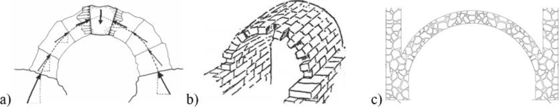
Figure 1. Several types of masonry arches used in historic buildings: a) voussoir system with ashlars (Huerta, S., 2006); b) voussoir system with ashlars (Heyman, J., 1995) c) irregular masonry vault with mortar (Segovia, M. A., 2022).
To glimpse the problems involved in analyzing historic buildings of unreinforced and irregular masonry, some researchers around the world who work on the subject are cited, to mention a few: Block, P., et. al., (2006), who state that graphical statics, interactive and limit analysis tools based on graphical statics provide methods to characterize and assess the structural stability of complex masonry systems that are efficient and fast to process, Chávez M., (2005/2010) has provided valuable information regarding the structural behavior of complete systems of heritage buildings and mechanical properties of masonry, modeled with continuous finite elements. On the other hand, Angelillo M., et al., (2014), has worked on structural analysis procedures of discretized historic masonry systems and elements, considering contact interaction between them. Durán D., et. al., (2022), who have studied the mechanical properties of ancient churches located in different parts of the world.
2. RECOGNITION OF THE STRUCTURAL SYSTEM OF THE HERITAGE OBJECT
The heritage object analyzed is a Mexican temple dating from the 16th century, located in the state of Hidalgo in the town of Santa Catarina, its original structure was made with irregular stones and earthen mortar from the site, it has 6 buttresses on the side walls, the latter serve as the base for the continuous barrel vault which is confined in its upper part by the site's land. Figure 2 shows the build before the integration of reinforced concrete elements and shows indications of its structural behaviour.
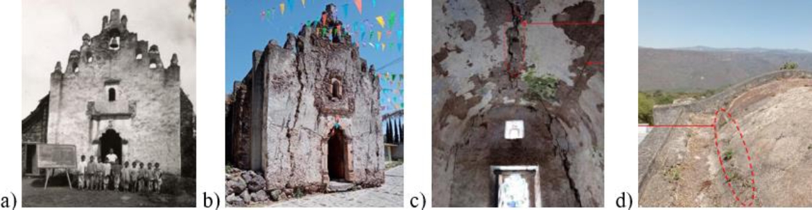
Figure 2. Temple of Santa Catarina; a) preserved building (Biblioteca Tomás Navarro Tomás, 2023); b) current state of the temple; c) and d) Cracks in the keystone and kidneys, respectively. Taken from (Segovia, M. A., 2022).
3. GEOMETRIC DISCRETIZATION OF SUBSYSTEMS
The strips with the highest susceptibility to lateral deformation are selected. Since they are not fully restrained by buttresses (see Figure 4).
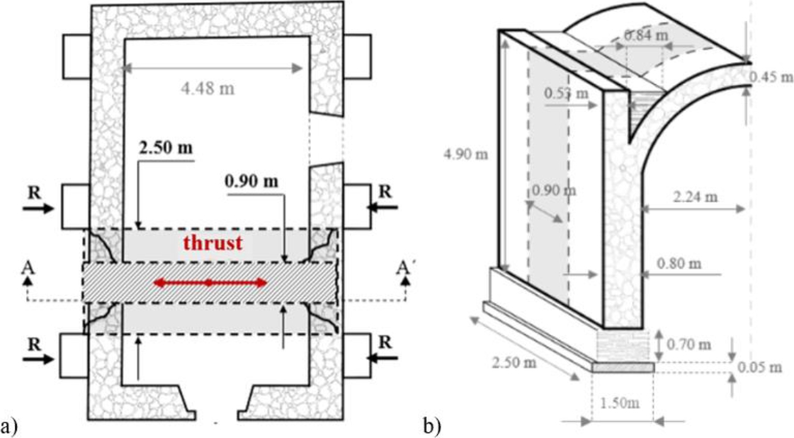
Figure 3. Strips selected for the analysis; a) plan view; b) Three-dimensional view of strips Fr1 and Fr2 with widths of 0.90m and 2.50m, respectively. Dimensions in meters.
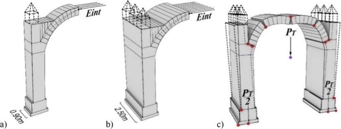
Figure 4. 3D view of Fr strips (subsystems) selected for analysis, a) subsystem Fr1 of 0.90m, b) subsystem Fr2 of 2.50m width, c) representation of the formation of hinges at specific points analogous to those of the real heritage object (see figure 3). Dimensions in meters.
At figure 4, in both systems the intermediate horizontal thrust (Eint) close to the minimum thrust (Emin) is exemplified (see figure 8). Theory taken from (Heyman, J., 1995; Huerta, S., 2004, Mas-Guindal; A. J., 2021).
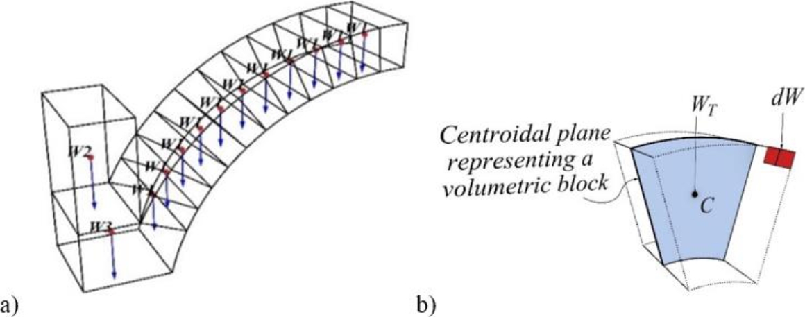
Figure 5. Centers of gravity of the blocks that form the system, a) gravitational forces concentrated on the discretized structural elements, b) total weight (WT) and differential weight (dW) of each atomised element, where: C = Center of gravity.
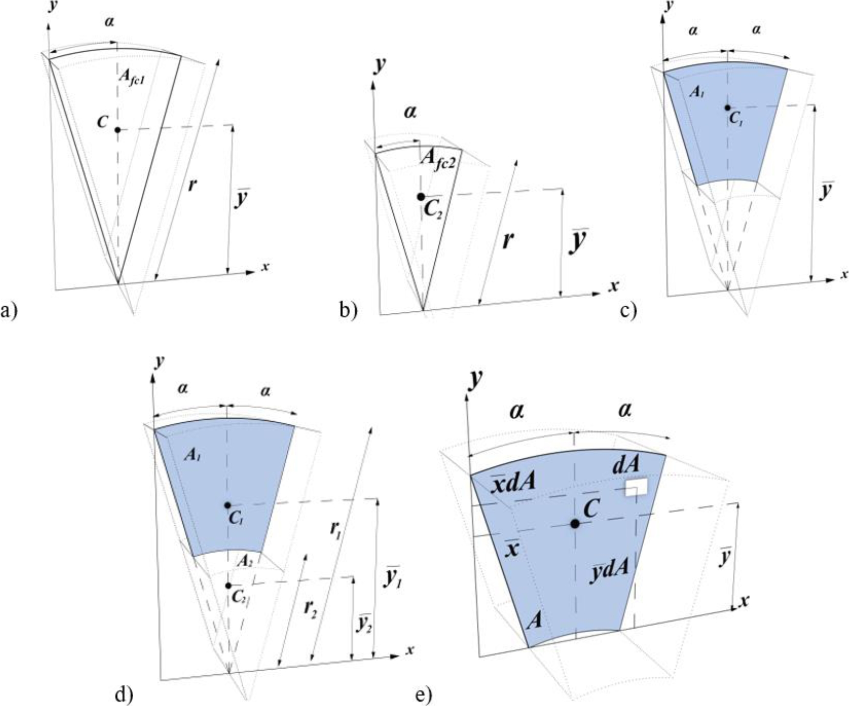
Fig. 6. Mathematical sequence to obtain the centers of gravity of the blocks, a) complete plane (Area) representative of the original shape, b) plane to be subtracted of the original shape, c) plane of the resulting segment, d) discretization of the geometric properties of the areas A1 y A2, e) Volumetric center of the block discretized block as the resulting segment.
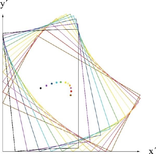
Fig. 7. Virtual discretization by blocks (voussoirs) of arch subsystem, where: EL: Discretized element, CE: Element colour, A = Area of the centroidal plane, i=1 to n, n= number of the discretized elements (11 for the arch subsystem of the object of the study, see figures 4 and 9).
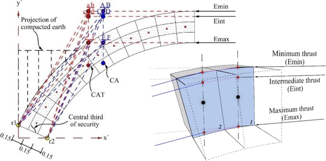
Fig. 8. Succession of vectors in each segment, generated by the lateral thrusts, illustrating the modification of the trajectories when intersecting the projection of the vertical line passing through the center of gravity of each element. Dimensions in meters; Subsystem arch and identification of possible thrust line and twist paths at the base of the vault.
Diagonal tension cracking at 45 degrees is adopted in walls, similar to unreinforced concrete (0; Meli, R. 2011). Unlike buildings currently constructed with continuous materials and construction systems, the formation of hinges does not represent stiffness degradation, but rather indicates the equilibrium points and behavioral patterns of the current physical conditions of the heritage object. The structural elements belonging to the selected strips are geometrically discretized (see figure 5), the geometry is modelled with the tendency of structural behaviour that the heritage object presents or has presented, to locate the contact points and therefore visualizing the conformation of possible hinges, which serves as a theoretical basis for generating the virtual divisions in the geometric models. The dotted lines are possible pinnacles to redirect the thrust vectors (see figures 6 and 10).
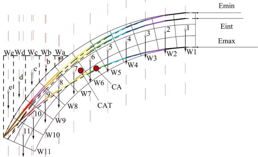
Fig. 9. Shows the location of the thrust lines when the arch subsystem tends to rotate with respect to the point "r1". It is worth mentioning that the rotation point "r1" was chosen since this is how the real object behaves (see figure 4c).
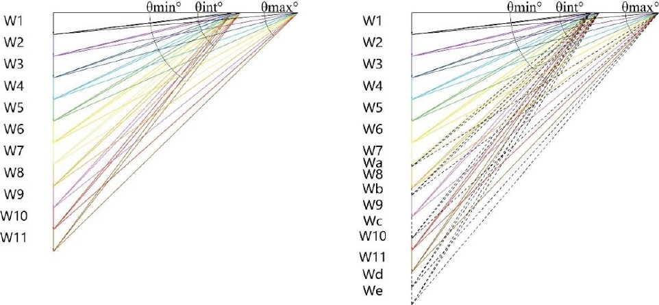
Fig. 9.1. Representation of dotted thrust lines, which consider the loads due to the earth placed on the dome. Table 3 shows the magnitudes of the thrusts in the subsystems: 1) arch and 2) arch with walls and foundation, both for the cases Emax, Eint, and Emin (see figure 10).
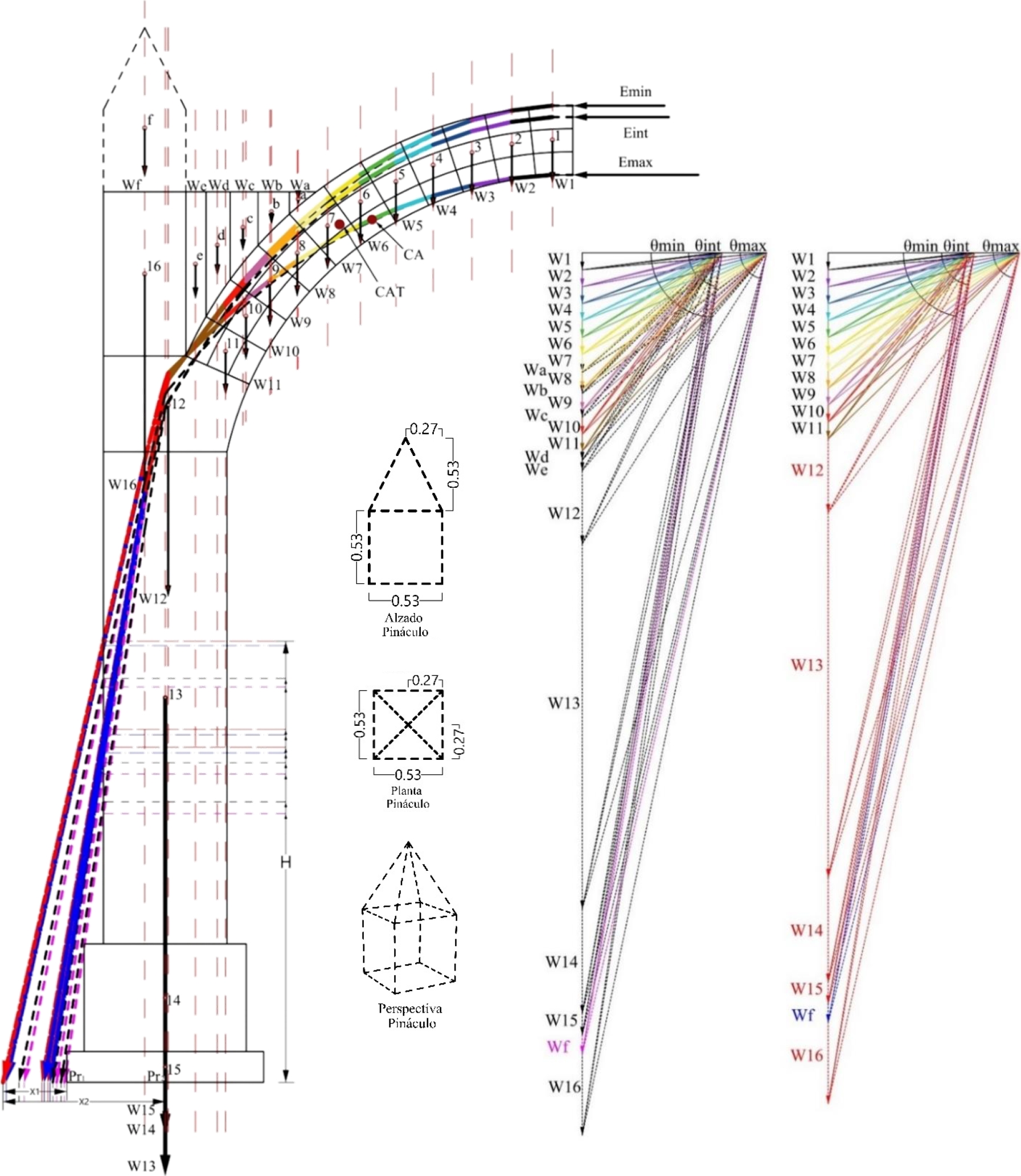
Figure 10. Vector analysis of the symmetrical subsystems, where the magnitudes and directions of the thrusts generated by all the elements, with and without the earth and pinnacle loads, can be observed.
4. NUMERICAL-VECTOR SUCCESSION OF THE SUBSYSTEM
Vector analysis consists of the representation of forces with certain magnitudes and directions that lead to a sequence of thrusts or reactions between the various volumetric elements (blocks) that make up the analyzed system; in this document, this analysis is used for the graphical representation of the gravity loads generated by each of the blocks (see figure 5) and for the simulation of the resulting vectors. In this analysis, mechanically homogeneous and isotropic elements with practically infinite resistance are considered, with no sliding between blocks and no tensile stresses, according to (Heyman, J. 1969; Huerta, S. 2004). Due to the fact, that the building has compacted earth, this is considered to have a density of 1,600 kg/m³, it is worth mentioning that this earth can take on other weights in rainy seasons, since the weight of the wet earth, according to (Minke, G. 1994) could increase to 1,800 kg/m³. Since the volumetric weight is essential to keep this type of structure in equilibrium, 2,700 kg/m³ is used, since, when determining the thrust lines with a lower parameter, they are out of the geometry (see fig. 10). The physical characteristics determined by (Chávez, Mauricio M. 2010), who found that the possible volumetric weight of irregular masonry joined with lime mortar is 1,627kg/m3.
At figure 5, the theory was taken and adapted from (Egor, P. P. and Toader, A. B. 1999; Goodno, B. J. and Gere, J. M., 2013; Hibbeler, R.C. 2016). Vector variables (W ⃗i) are represented with an arrow according to (Spiegel, M. R. 1970).
Since the discretized element is isotropic and homogeneous, its total weight is the sum of the differential weights (see equation 1 and fig. 6b). (Hibbeler, R.C. 2016) mentions that, if a body is made of a homogeneous material, it has a constant density and the force generated by the weight of the body passes through a volumetric center (center of gravity). Applying these principles to the object presented in figure 5a, it is possible to visualize the gravitational vectors intersecting with the center of gravity of each homogeneous and discretized element. Figure 6 illustrates the mean planes and their mathematical support for locating and representing the centers of gravity of voussoir-type volumetric elements, idealized as flat elements (areas). Equations (2)-(7) define the above; by applying these mathematical expressions, both the surfaces of the discretized block planes representing the segments and the ordinates of their centers of gravity are determined. The center of gravity is calculated with first order moments (Egor, P. P. and Toader, A. B. 1999; Goodno, B. J. and Gere, J. M. 2013).
| (1) |
| (2) |
| (3) |
| (3´) |
| (4) |
| (5) |
| (6) |
| (7) |
Where: dW= differential weight of the element, = Total Weight of the element, x= distance since “x” axis to the centroid of dA, y= distance since “y” axis to the centroid of dA, dA= differential area, i=1 to n, n= number of the discretized elements, A= total area, = cone area, α= angle, r= radius of circular sector.
At figure 6, Afc= Area of conical shape, C1= Center of gravity of A1, C2= Center of gravity of A2, A1= Area that remains after subtraction, A2= Area that is subtracted, α= Opening angle (in degrees) of the circular sector to centroidal axis, g= conical generatrix, 1= Distance from “x” axis to the centroid of A1, 2= Distance from “x” axis to the centroid of A2, A= Resultant area, C= Center of gravity of A, dA= Partial area r= radius, The angle α is affected by (π/180) to convert to radians.
With the numerical expressions shown in figure 6, the geometric properties for the analysis of the arch subsystem are obtained (see figure 7). In figure 6 the discretized elements (voussoirs) are superimposed to differentiate the center of gravity based on their position referred to local axes (x’, y'), however, for this case all the elements of the arch subsystem have the same volumetric weight (see table 1). The thrust line modifies its trajectory successively when it virtually intersects the vertical line of the center of gravity of each segment. In the case where the compression line leaves the geometry, it means that the compression would be outside the element and therefore the blocks would no longer be in contact with each other in that section. The minimum thrust is represented as a horizontal force in the upper zone of the segments commonly referred to as the keystone. In the case of a symmetrical gravity system, it is sufficient to analyze one half (see figure 9) to know the trajectory of the compression thrust line, so it is essential to adequately determine the gravity loads and centers of gravity of each of the blocks since the correct generation of the thrust between adjacent blocks depends on this.
Table 1. Numerical centers of gravity and colour coding of the discretized segments to make up the arch subsystem (see figure 7).
| ELi | CEi | ´i (m) | ´i (m) |
| 1 | 0.1547 | 0.2397 | |
| 2 | 0.1756 | 0.2496 | |
| 3 | 0.1945 | 0.2568 | |
| 4 | 0.2114 | 0.2612 | |
| 5 | 0.2259 | 0.2627 | |
| 6 | 0.2379 | 0.2614 | |
| 7 | 0.2473 | 0.2572 | |
| 8 | 0.2541 | 0.2501 | |
| 9 | 0.2580 | 0.2402 | |
| 10 | 0.2591 | 0.2280 | |
| 11 | 0.2571 | 0.2127 |
To determine the trajectory of the thrust line, emanating from the arc-type subsystem, it is necessary to select the exact and/or the most critical possible location according to the state of the real physical object. In case of developing the analysis with the minimum critical thrust, i.e. indicating a horizontal vector in the upper zone, practically intersecting the vertex, it would mean that such a subsystem is in imminent collapse. To determine the trajectory of the thrust line, the funicular polygon and polygon of forces can be used to provide the flow of forces in the structural elements of systems with alternative shapes (Markou, A. A. and Ruan, G. 2022). Figure 8 shows the minimum horizontal thrust and the modification of its trajectory in each element (block), due to the interaction with the forces acting on the centers of gravity. Table 2 shows the properties that represent and configure each element of the Fr1 and Fr2 systems with walls and foundations.
Table 2. Magnitudes and angles of the vectors in the earthless arc subsystem.
| Earthless arc subsystem | |||||||||
| Element | Emax | Eint | Emin | ||||||
| Vri (Kg) | θ°max | Vri (Kg) | θ°int | Vri (Kg) | θ°min | ||||
| Fr1 | Fr2 | Fr1 | Fr2 | Fr1 | Fr2 | ||||
| EL | 3,248.85 | 9,024.58 | 0 | 2,464.03 | 6,844.53 | 0 | 2,350.48 | 6,529.11 | 0 |
| 1 | 3,261.63 | 9,060.08 | 5.07 | 2,480.85 | 6,891.25 | 6.68 | 2,368.11 | 6,578.08 | 7 |
| 2 | 3,299.67 | 9,165.75 | 10.07 | 2,530.66 | 7,029.61 | 13.18 | 2,420.24 | 6,722.89 | 13.79 |
| 3 | 3,362.11 | 9,339.19 | 14.91 | 2,611.55 | 7,254.31 | 19.35 | 2,504.70 | 6,957.50 | 20.21 |
| 4 | 3,447.63 | 9,576.75 | 19.55 | 2,720.77 | 7,557.69 | 25.09 | 2,618.38 | 7,273.28 | 26.15 |
| 5 | 3,554.57 | 9,873.81 | 23.94 | 2,855.06 | 7,930.72 | 30.34 | 2,757.66 | 7,660.17 | 31.53 |
| 6 | 3,681.05 | 10,225.14 | 28.04 | 3,011.07 | 8,364.08 | 35.08 | 2,918.88 | 8,108.00 | 36.36 |
| 7 | 3,825.14 | 10,625.39 | 31.86 | 3,185.61 | 8,848.92 | 39.33 | 3,098.62 | 8,607.28 | 40.63 |
| 8 | 3,984.93 | 11,069.25 | 35.39 | 3,375.81 | 9,377.25 | 43.12 | 3,293.85 | 9,149.58 | 44.47 |
| 9 | 4,158.61 | 11,551.69 | 38.63 | 3,579.17 | 9,942.14 | 46.49 | 3,501.97 | 9,727.69 | 47.84 |
| 10 | 4,344.52 | 12,068.11 | 41.60 | 3,793.58 | 10,537.72 | 49.49 | 3,720.83 | 10,335.64 | 50.82 |
| 11 | 4541.14 | 12,614.28 | 44.32 | 4,017.26 | 11,159.06 | 52.17 | 3,948.64 | 10,968.44 | 53.47 |
At figure 8, Emin= Minimum thrust, Eint= Intermediate thrust, Emax= Maximum thrust, r1-r2: rotation points. Nodes (a)-(f): intersections between the vertical line passing through the centroid of the compacted earth arch subsystem and the vector thrusts. Nodes (A)-(F): intersections between the vertical line through the centroid of the earth-free arch subsystem and the vector thrusts. CA and CAT: centers of gravity of the earthless arch and compacted earth subsystems, respectively. Theory taken of (Barlow, William Henry 1846; Meli, R. 1998).
Where: Emax= Maximum thrust, Eint= Intermediate thrust, Emin= Minimum thrust, Vr= Trust vector belonging to element “i” (represented with magnitude), i=1 to n, n= Discretized elements number, Eh= Horizontal thrust θ= Angle in degrees. Fr1 y Fr2, structural systems with thickness of 0.90m and 2.50m, respectively.
Where: EL= Discretized element, A = Area of the centroidal plane, i =1 to n, n= number of discretized elements, V= Volume, W= Gravity load, W ⃗= Magnitude of the vector representing the gravity load. Fr1 and Fr2, structural subsystems with widths of 0.90m and 2.50m, respectively.
The shaded rows represent the discrete earth elements above the vault (see figures 8b and 9a). The values referring to the letter "f" represent the pinnacle elements, where cases Fr1 and Fr2 have one and three pinnacles, respectively (see figure 10). Figure 10 and table 4 present the analysis and results for the symmetric subsystems (with wall and foundation) for the cases with and without earth on top of the vault, and with and without pinnacles.
Table 3. Numerical-vector values of the physic-geometric properties of subsystems Fr1 and Fr2, successively ordered for the vector analysis.
| ELi | xi |
yi |
Ai |
Vi |
Wi |
||||
| Fr1 | Fr2 | Fr1 | Fr2 | Fr1 | Fr2 | ||||
| 1 | 0.1547 | 0.2397 | 0.1187 | 0.1068 | 0.2968 | 288.44 | 801.23 | 28.84 | 80.12 |
| 2 | 0.1756 | 0.2496 | |||||||
| 3 | 0.1945 | 0.2568 | |||||||
| 4 | 0.2114 | 0.2612 | |||||||
| 5 | 0.2259 | 0.2627 | |||||||
| 6 | 0.2379 | 0.2614 | |||||||
| 7 | 0.2473 | 0.2572 | |||||||
| a | 0.0573 | 0.0969 | 0.0122 | 0.0110 | 0.0306 | 17.61 | 48.91 | 1.76 | 4.89 |
| 8 | 0.2541 | 0.2501 | 0.1187 | 0.1068 | 0.2968 | 288.44 | 801.23 | 28.84 | 80.12 |
| b | 0.0874 | 0.2192 | 0.0492 | 0.0443 | 0.1230 | 70.87 | 196.87 | 7.09 | 19.69 |
| 9 | 0.2580 | 0.2402 | 0.1187 | 0.1068 | 0.2968 | 288.44 | 801.23 | 28.84 | 80.12 |
| 10 | 0.2591 | 0.2280 | |||||||
| c | 0.0830 | 0.3386 | 0.0822 | 0.0740 | 0.2056 | 118.44 | 328.99 | 11.84 | 32.90 |
| 11 | 0.2574 | 0.2139 | 0.1187 | 0.1068 | 0.2968 | 288.44 | 801.23 | 28.84 | 80.12 |
| d | 0.0736 | 0.4648 | 0.1074 | 0.0966 | 0.2684 | 154.62 | 429.50 | 15.46 | 42.95 |
| e | 0.0622 | 0.5975 | 0.1218 | 0.1096 | 0.3044 | 175.35 | 487.08 | 17.53 | 48.71 |
| 12 | 0.4188 | 0.3036 | 0.5147 | 0.4633 | 1.2868 | 1250.79 | 3474.42 | 125.08 | 347.44 |
| 13 | 0.4000 | 1.6000 | 2.5600 | 2.3040 | 6.4000 | 6220.80 | 17280.01 | 622.08 | 1728.00 |
| 14 | 0.5250 | 0.3500 | 0.7350 | 0.6615 | 1.8375 | 1786.05 | 4961.25 | 178.61 | 496.13 |
| 15 | 0.6375 | 0.1000 | 0.2550 | 0.2295 | 0.6375 | 367.20 | 1020.00 | 36.72 | 102.00 |
| f | 0.2667 | 0.4149 | 0.4268 | 0.2024 | 0.6072 | 323.82 | 971.45 | 32.38 | 97.14 |
| 16 | 0.2667 | 0.5337 | 0.5694 | 0.5124 | 1.4235 | 1383.61 | 3843.36 | 138.36 | 384.34 |
Table 4. Magnitudes and angles of thrusts per element in the symmetric system with wall and foundation for the twelve possible thrust line trajectories presented in figure 10.
| Symmetrical unearthed and earthed subsystem above the dome | |||||||||
| Element | Emax | Eint | Emin | ||||||
| Vri (Kg) | θ°max | Vri (Kg) | θ°int | Vri (Kg) | θ°min | ||||
| Fr1 | Fr2 | Fr1 | Fr2 | Fr1 | Fr2 | ||||
| EH | 3,135.70 | 8,710.28 | 0 | 2,378.21 | 6,606.14 | 0 | 2,268.62 | 6,301.72 | 0 |
| 1 | 3,148.94 | 8,747.06 | 5.26 | 2,395.64 | 6,654.56 | 6.92 | 2,286.88 | 6,352.44 | 7.25 |
| 2 | 3,188.33 | 8,856.47 | 10.42 | 2,447.18 | 6,797.72 | 13.64 | 2,340.82 | 6,502.28 | 14.27 |
| 3 | 3,252.91 | 9,035.86 | 15.43 | 2,530.75 | 7,029.86 | 19.99 | 2,428.05 | 6,744.58 | 20.88 |
| 4 | 3,341.23 | 9,281.19 | 20.20 | 2,643.31 | 7,342.53 | 25.88 | 2,545.15 | 7,069.86 | 26.96 |
| 5 | 3,451.46 | 9,587.39 | 24.70 | 2,781.34 | 7,725.94 | 31.23 | 2,688.23 | 7,467.31 | 32.44 |
| 6 | 3,581.59 | 9,948.86 | 28.90 | 2,941.26 | 8,170.17 | 36.04 | 2,853.38 | 7,926.06 | 37.34 |
| 7 | 3,729.52 | 10,359.78 | 32.78 | 3,119.71 | 8,665.86 | 40.33 | 3,037.00 | 8,436.11 | 41.67 |
| a | 3,739.09 | 10,386.36 | 33.00 | 3,131.14 | 8,697.61 | 40.58 | 3,048.73 | 8,468.69 | 41.92 |
| 8 | 3,903.70 | 10,843.61 | 36.56 | 3,325.98 | 9,238.83 | 44.35 | 3,248.52 | 9,023.67 | 45.70 |
| b | 3,946.33 | 10,962.03 | 37.38 | 3,375.91 | 9,377.53 | 45.21 | 3,299.62 | 9,165.61 | 46.56 |
| 9 | 4,127.82 | 11,466.17 | 40.57 | 3,586.39 | 9,962.19 | 48.46 | 3,514.67 | 9,762.97 | 49.80 |
| c | 4,205.81 | 11,682.81 | 41.79 | 3,675.88 | 10,210.78 | 49.69 | 3,605.94 | 10,016.50 | 51.01 |
| 10 | 4,403.29 | 12,231.36 | 44.59 | 3,900.28 | 10,834.11 | 52.43 | 3,834.44 | 10,651.22 | 53.73 |
| 11 | 4,610.37 | 12,806.58 | 47.15 | 4,132.64 | 11,479.56 | 54.87 | 4,070.56 | 11,307.11 | 56.13 |
| d | 4,724.89 | 13,124.69 | 48.42 | 4,260.03 | 11,833.42 | 56.06 | 4,199.83 | 11,666.19 | 57.30 |
| e | 4,857.45 | 13,492.92 | 49.79 | 4,406.59 | 12,240.53 | 57.34 | 4,348.43 | 12,078.97 | 58.55 |
| 12 | 5,865.52 | 16,293.11 | 57.68 | 5,501.16 | 15,281.00 | 64.39 | 5,454.68 | 15,151.89 | 65.42 |
| 13 | 11,612.70 | 32,257.50 | 74.33 | 11,431.45 | 31,754.03 | 77.99 | 11,409.15 | 31,692.08 | 78.53 |
| 14 | 13,341.12 | 37,058.67 | 76.41 | 13,183.66 | 36,621.28 | 79.61 | 13,164.33 | 36,567.58 | 80.08 |
| 15 | 13,698.31 | 38,050.86 | 76.77 | 13,545.00 | 37,625.00 | 79.89 | 13,526.19 | 37,572.75 | 80.34 |
| f | 14,013.73 | - | 77.07 | 13,863.90 | - | 80.12 | 13,845.52 | - | 80.57 |
| f | - | 40,682.39 | 77.64 | - | 40,284.36 | 80.56 | - | 40,235.56 | 80.99 |
| 16 | 15,365.37 | - | 78.22 | 15,228.85 | - | 81.02 | 15,212.12 | - | 81.42 |
| 16 | - | 44,444.25 | 78.70 | - | 44,080.19 | 81.38 | - | 44,035.61 | 81.77 |
Where: Emax= Maximum thrust, Eint= Intermediate thrust, Emin= Minimum thrust, Vr= Thrust vector belonging to element “i”, i=1 ton, n= discretized element number, EH= horizontal element, θ= Angle. Fr1 y Fr2, structural systems with thickness of 0.90m and 2.50m, respectively.
At figure 10 the vectors representing the loads W13, W14 and W15 are scaled by half and their thickness is doubled so that they to still have a graphically representative magnitude. In this figure only the vector analysis for Fr1 is shown. Dimensions in meters. Note: The black dotted line without arrow at the end represents the calculated thrust with a volumetric weight of the masonry of 1,627kg/m3, which comes out of the geometry.
Figure 11 shows the possible foundation overturning moments. Table 5 shows the magnitudes and ratios of the acting (Mv) and resisting (Mr) overturning moments according to the resulting vectors for the different subsystems (see figure 10). Mv= Overturning moment, GI= Initial rotation, GF= Final rotation, K= Vertical stiffness of soil. Theory taken from (Meli, R. 2011) and adapted by the author.
Fig. 11. Overturning moments according to the behaviour of the foundation in different soil types. a) foundation placed on non-compressible soil, b) foundation placed on medium compressible soil, c) foundation placed on highly compressible soil.
Table 5. Results of the different thrust lines in the symmetric subsystems with wall and foundation for the twelve possible configurations analyzed for Fr1.
| ELEMENT | Vuri |
Py |
H |
X1 |
X2 |
θ° | Mv1 |
Mr/Mv1 |
Mv2 |
Mr/Mv2 |
||
| Emin | c/t | c/p | 15,212.12 | 14,916.55 | 2.57 | 0.28 | 0.92 | 78.69 | 4,176.63 | 200 | 13,723.23 | 61 |
| s/p | 14,892.00 | 14,578.04 | 2.63 | 0.31 | 0.95 | 78.21 | 4,519.19 | 184 | 13,849.13 | 60 | ||
| s/t | c/p | 14,697.62 | 14,347.17 | 2.84 | 0.29 | 0.93 | 77.46 | 4,160.68 | 200 | 13,342.87 | 62 | |
| s/p | 14,378.13 | 14,020.16 | 2.87 | 0.41 | 1.05 | 77.19 | 5,748.26 | 145 | 14,721.16 | 57 | ||
| Eint | c/t | c/p | 15,228.85 | 15,056.43 | 2.01 | 0.07 | 0.71 | 81.37 | 1,053.95 | 791 | 10,690.06 | 78 |
| s/p | 14,909.09 | 14,725.74 | 2.08 | 0.09 | 0.73 | 81.01 | 1,325.32 | 629 | 10,749.79 | 78 | ||
| s/t | c/p | 14,716.36 | 14,508.00 | 2.26 | 0.15 | 0.79 | 80.35 | 2,176.20 | 383 | 11,461.32 | 73 | |
| s/p | 14,397.29 | 14,184.28 | 2.29 | 0.16 | 0.80 | 80.13 | 2,269.49 | 367 | 11,347.43 | 73 | ||
| Emax | c/t | c/p | 15,365.37 | 15,206.82 | 1.75 | 0.02 | 0.66 | 81.76 | 304.14 | 2740 | 10,036.50 | 83 |
| s/p | 15,048.51 | 14,879.78 | 1.82 | 0.04 | 0.68 | 81.41 | 595.19 | 1400 | 10,118.25 | 82 | ||
| s/t | c/p | 14,864.51 | 14,672.47 | 2.14 | 0.11 | 0.75 | 80.78 | 1,613.97 | 516 | 11,004.35 | 76 | |
| s/p | 14,570.44 | 14,373.71 | 2.18 | 0.12 | 0.76 | 80.57 | 1,724.85 | 483 | 10,924.02 | 76 | ||
On the other hand, computerized analyses were also developed by means of software (Computers and Structures, Inc. 2023), based on the Finite Element Method (FEM). Figures 12 to 17 show the simulations of the structural behavior of Fr1 strips, which consider the continuous and discontinuous structure. In the discontinuous models, the finite element spacings were simulated in the cracked areas of the vault in the real object. In the continuous models, no such gaps were simulated. For the modeling, flat shell-type and 3D solid-type elements were taken into account. According to (Circolare, 2019), the elastic modulus (E), for all models, was taken as 7036 kg/cm2. Poisson's modulus of 0.17. The density of the materials was considered the same as in the graphical analyses.
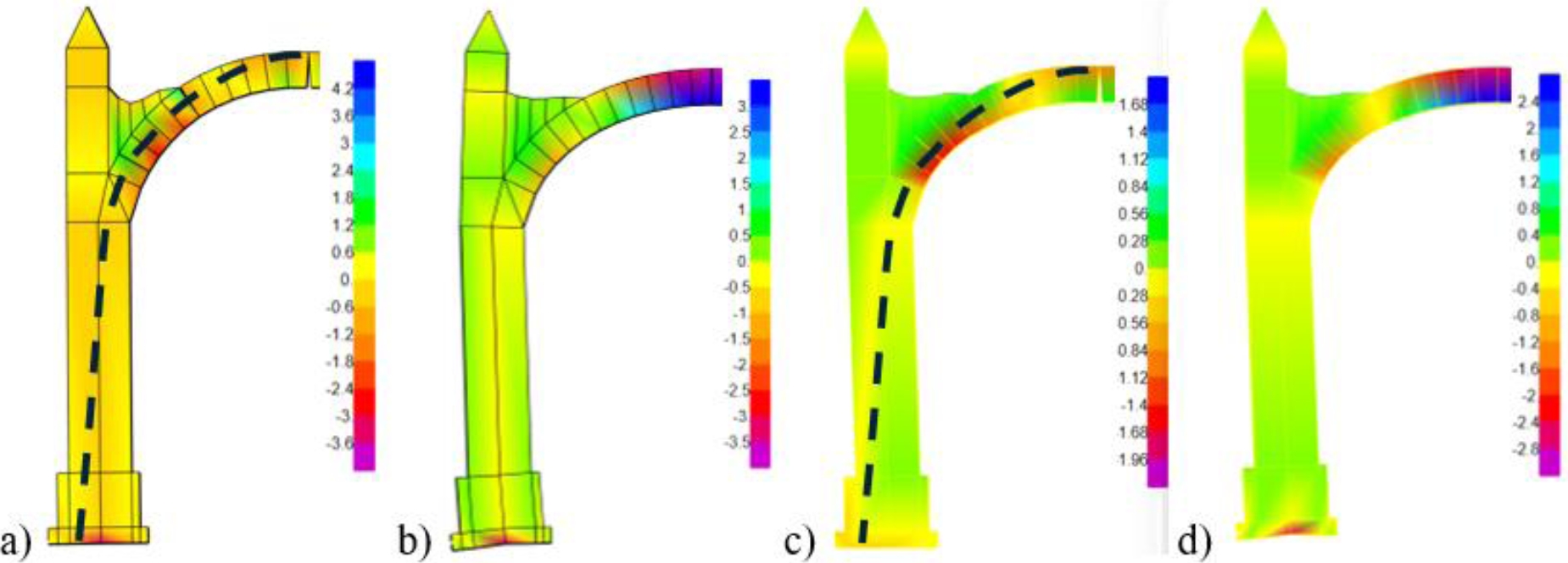
Fig. 12. Stresses in kg/cm2 and deformation behavior in the symmetrical half with pinnacles, earth filling on top of vault and with free rotation at the center of the foundation. Cases: a) discontinuous with shell. b) continuous with shell. c) discontinuous with solids. d) continuous with solids.
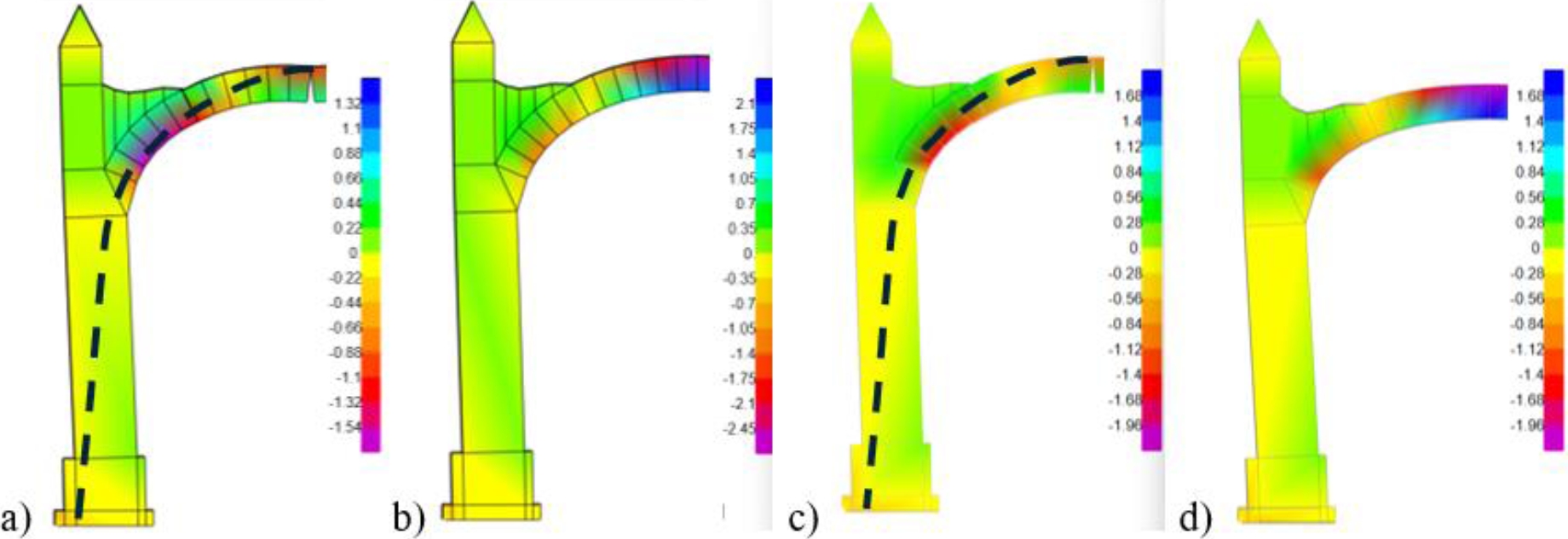
Figure 13. Stresses in kg/cm2 and deformation behavior in the symmetrical half with pinnacles, earth filling on top of vault and with total support of the foundation. Cases: a) discontinuous with shell. b) continuous with shell. c) discontinuous with solids. d) continuous with solids.
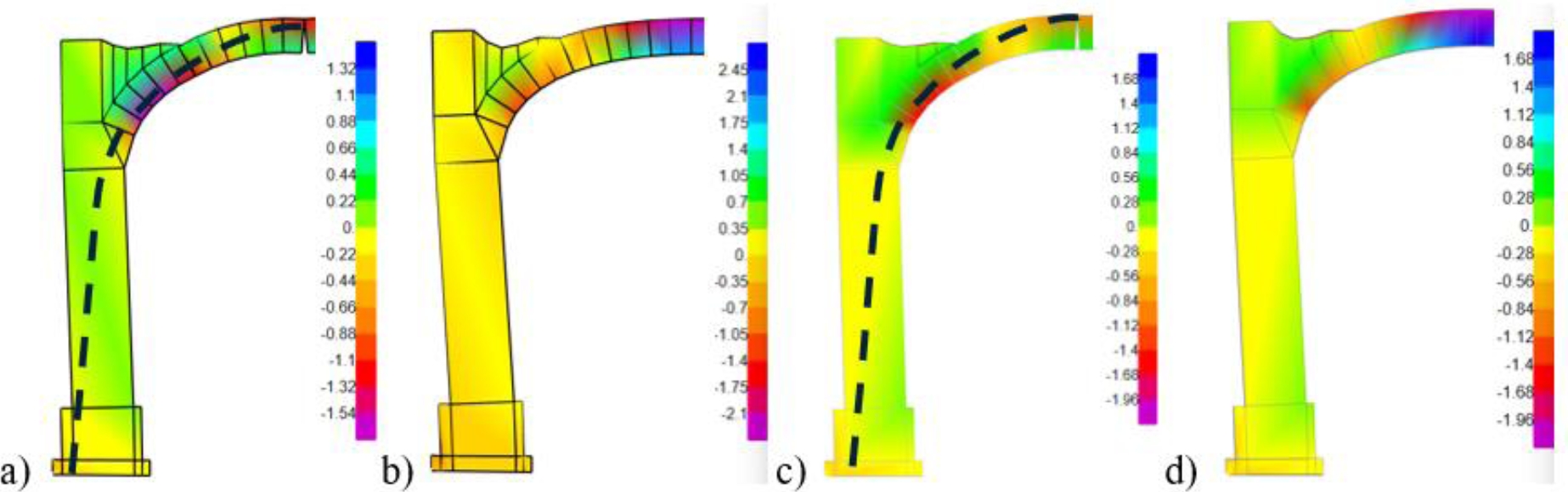
Figure 14. Stresses in kg/cm2 and deformation behavior in the symmetrical half without pinnacles, with earth filling on top of vault and free rotation at the center of the foundation. Cases: a) discontinuous with shell. b) continuous with shell. c) discontinuous with solids. d) continuous with solids.
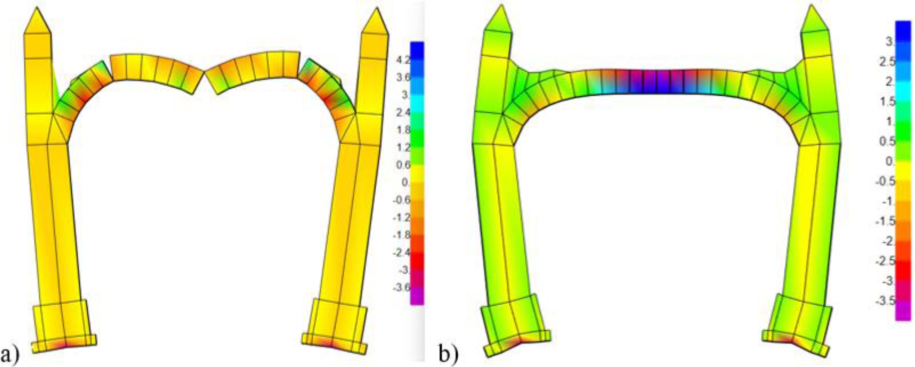
Figure 15. Virtual simulation of complete Fr1 strip of structural behavior by means of finite elements. a) Fr1 strip modeled with discontinuous shell elements according to the problems presented by the real object. b) Fr1 strip modeled with continuous shell elements. Both models allow rotation in the foundation.
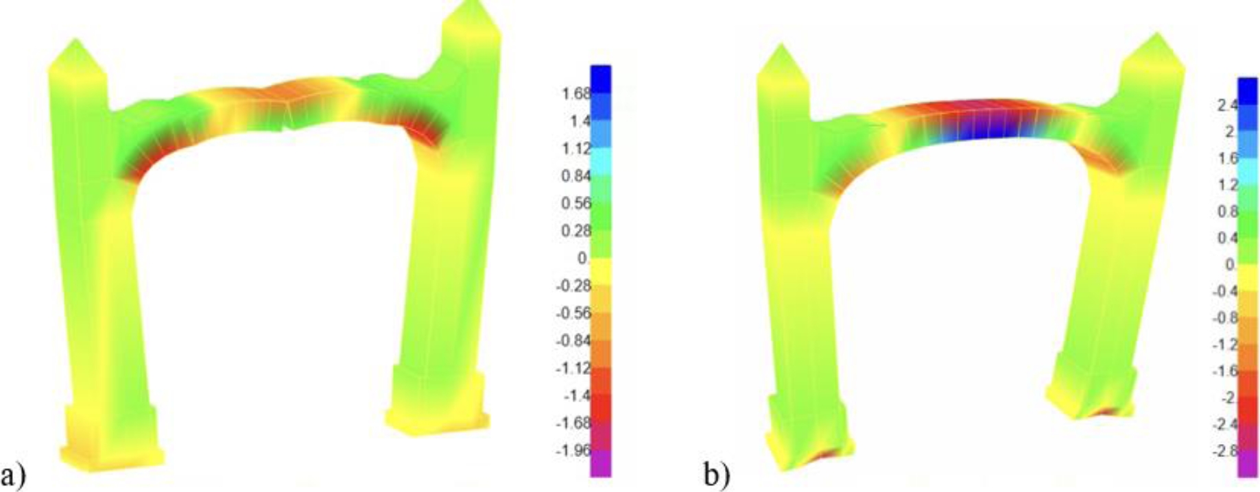
Figure 16. Virtual simulation of complete Fr1 strip of structural behavior by means of finite elements. a) Fr1 strip modeled with discontinuous solid type elements according to the problems presented by the real object. b) Fr1 strip modeled with continuous solid type elements. Both models allow rotation in the foundation.
The Fr1 fringe models shown in Figure 15a and 15b present periods of vibration in the direction parallel to the plane of T=0.1 s and T=0.51 s respectively, both cases, were carried out with the foundation base simply supported.
As can be seen in figures 13 to 16, the compression lines do not leave the geometry of the structures, since these finite element models tend to develop equilibrium between tension and compression in continuous elastic materials.
5. RESULTS AND DISCUSSION
The application of mathematical equations and their computational processing decreased the time of graphic strokes, given that in the same systematized strip twelve different possibilities of structural behaviour were developed and the results were more accurate, given the precision required by vector analysis. The process of analysis of historic masonry buildings with arches and symmetrical systems presented in this work can be applied in research and professional practice quickly and accurately, to find the necessary loads to maintain structural static equilibrium. Mathematical process to determine the voussoir areas are based on completely curves arches, in case of required analyze arches with straight segments, these mathematical equations should be changed.
Where: Py= Vertical component of the ultimate vector (Vuri), H= height measured from the contact surface of the foundation with the ground to the intersection of the ultimate vector (Vuri) with the perimeter (boundary) line of the wall (Element 13 for this object of study), X= measured dimension of the overturning point at Py, Mv1= overturning moment in very hard soil, Mv2= overturning moment in very soft soil, Mr= resisting moment= 8334 kg-m, s/t= without earth, s/p= without pinnacles, c/t= with earth, c/p= with pinnacles. In this table only the results of the Fr1 system are presented, as they are proportional according to the width of the strips.
When comparing the results of the graphic analysis with those obtained by finite element analysis, it can be observed that the structural behavior tends to be similar, but with some particularities, the walls tend to rotate outwards and the vault is prone to drop, where the top of the keystone moves downwards due to gravitational effects. In the elements modeled as discontinuous, the soffit of the keystone tends to stress and since the masonry has very little tensile strength, even if they are voussoirs, that zone opens causing a twist in the upper contact zone or point and thus generating what in graphic methods is called minimum horizontal thrust (Emin). The results that most closely resemble the graphical method are the models with shell-type elements where the discontinuity is considered as it is in the real object. For example: when comparing the forces calculated with the graphical static method in the case where discontinuity was considered, earth above the vault and pinnacle, a minimum horizontal thrust of 2268.62kg was obtained (see table 4), and in the same case modeled with finite elements, a stress in the same zone of 0. 33kg/cm2, therefore, when converted into force, a horizontal thrust of 2970kg was obtained (see figure 12a), therefore, the Emin calculated with graphic methods, for this particular case, had a difference of 24% less in magnitude than the one calculated with finite elements, this is due to the redistribution of mechanical elements and forces due to the continuity of the system based on shells or solids. On the other hand, to determine the thrust line in the finite element models, each surface delta of each modeled shell element was selected to find the compression that represents the thrust line in order to plot it.
6. CONCLUSIONS
In homogeneous, isotropic, infinitely strong structural systems with no slip between elements, only the symmetric half can be modelled. The selection of the rotation points of the arched subsystem is conditioned by the configuration the structure has, has had, or will have. The more virtual or real divisions the system has, the greater the accuracy in determining and shaping the hinges and, therefore, the greater the certainty in obtaining the position of the thrust line.
The type of soil contributes to the behaviour of the superstructure, as second order effects (P-Delta) can be generated, due to possible overturning of the foundation. The contribution of the loads from the pinnacles at the top of the walls and from the earth at the top of the vault results in a higher stability against overturning effects on walls and foundations, in particular the presence of the load due to the earth, relocates the thrust line closer to the geometric central third of safety in the arch subsystem. The integration of pinnacles and earth considerably increased the Resistant Moment / Overturning Moment ratio.
When comparing the compression thrust lines of the graphical and finite element models, it is evident that there are some differences, since the finite elements used in these analyses have continuity in most of the models, since most of them are continuous and present tractions. It is concluded that these methods provide very particular results and some of them are similar, therefore, it is recommended to use the methods as a complement and not to catalogue one over the other. Finally, it is important to study this type of structures with contact element analysis.
7. ACKNOWLEDGEMENTS
Grateful to Jorge Fernando Zárate Martínez for his support in the final proofreading in English. Thanks also to Elizabeth Amador for facilitating access to the building. To Academic Unit Escuela Superior de Ingeniería y Arquitectura Unidad Tecamachalco (ESIA UT) of Instituto Politécnico Nacional (IPN), México.
8. REFERENCES
Angelillo, M. et al. (2014), “Mechanics of Mansory Structures”, Editado por Maurizio Angelillo. Springer. Università di Salerno, Fisciano, Italy.
Biblioteca Tomás Navarro Tomás (19/10/2023), “Escuela de Santa Catarina, Atotonilco El Grande en Hidalgo (México)”, https://www.pinterest.com.mx/pin/334533078561349371/
Barlow, William Henry (1846). "On the Existence (practically) of the line of equal Horizontal Thrust in Arches, and the mode of determining it by Geometrical Construction “, Minutes and Proceedings of the Institution of Civil Engineers, Vol. 5, pp. 179-180.
Block, P., DeJong, M., Ochsendorf, J. A. (2006), "As Hangs the Flexible Line: Equilibrium of Masonry Arches". Nexus Network Journal - Vol 8, No. 2. https://doi.org/10.1007/s00004-006-0015-9.
Chávez, Mauricio M. (2010), “Validación Experimental De Modelos Analíticos Para El Estudio Del Comportamiento Sísmico De Estructuras Históricas”, México, UNAM, p. 24.
Chávez, M. (2005), “Estudio experimental de las propiedades mecánicas de mamposterías de piedra natural”, publicado por el Instituto de ingeniería UNAM. Ciudad Universitaria, CP 04510, Ciudad de México.
Chávez, M. (2010), “Validación experimental de modelos analíticos para el estudio del comportamiento sísmico de estructuras históricas”, publicado por el Instituto de Ingeniería UNAM. Ciudad Universitaria, CP 04510, Ciudad de México.
Circolare (2019), Código italiano DM 14.1. Il Ministro: Toninelli
Durán, D., Chávez, m. M. (2022), "Mechanical properties of masonry stone samples extracted from Mexican colonial churches", Elsevier, coordinación de ingeniería estructural, instituto de ingeniería, universidad nacional autónoma de México, México, E01295, https://doi.org/10.1016/j.cscm.2022.e01295
Goodno, B. J., Gere, J. M., (2013), “Mechanics of Materials (Ninth Edition)”, Cengage Learning, U.S., pp. 26-27.
Mas-Guindal, A. J. (2021). “Mecánica de las estructuras antiguas o cuando las estructuras no se calculaban”. Munilla-Lería, España-Madrid.
Heyman, J. (1969), “Teoría, Historia Y Restauración De Estructuras De Fábrica”, Inst. Juan de Herrera, México, pp. 1-1
Heyman, J. (1995), “The Stone Skeleton Structural engineering of masonry architecture (First Publish)”, Cambridge University Press, United Kingdom, pp. 5-49.
Hibbeler, R.C. (2016), “Ingeniería mecánica estática (decimosegunda edición)”, Prentice Hall, Pearson Educación, México, pp. 447-456, 599.
Huerta, S. (2004), “Arcos, bóvedas y cúpulas. Geometría y equilibrio en el cálculo tradicional de estructuras de fábrica”, Inst. Juan de Herrera, Madrid, pp. 11-34.
Huerta, S. (2006). “Galileo was wrong: The Geometrical Design of Masonry Arches”, E.T.S. de Arquitectura Universidad Politécnica de Madrid, Inst. Juan de Herrera, Nexus Network Journal 8 (2006), p. 26.
ICOMOS Internacional Council of Monument and Cities. (2003). “Principles for the analysis, conservation, and restoration of architectural heritage structures”. Victoria Falls, Zambia. Retrieved from http://www.icomos.org
ISCARSAH. (2003). “Recommendations for the analysis conservation, and structural restoration of architectural heritage”. Course on Architectural Heritage Intervention of the College of Architects of Catalonia. Catalonia: ICOMOS.
Markou, A. A., Ruan, G. (2022), “Graphic statics: projective funicular polygon”, ELSEVIER, Department of Civil Engineering, Aalto University, Rakentajanaukio 4A, Espoo FI-00076, Finland, pp. 1394-1395.
Mas-Guindal, A. J. (2021). “Mecánica de las estructuras antiguas o cuando las estructuras no se calculaban”. Munilla-Lería, España-Madrid, pp. 34-73.
Mc Cormac, J. C., Brown, R. H. (2017), “Diseño de Concreto Reforzado (décima edición)”, Alfaomega Grupo Editor, México, p. 355.
Meli, R. (1998), “Ingeniería estructural de los edificios históricos”, ICA, México, p. 10
Meli, R. (2011), “Diseño Estructural (segunda edición)”, Limusa Noriega Editores, México, p. p. 544, 552.
Minke, G. (1994), “Manual de construcción en tierra, La tierra como material de construcción y su aplicación en la arquitectura actual”, Editorial Fin de Siglo, Alemania, p. 25.
Popov, E. P., Toader, A. B. (1999),” Mecánica de Sólidos (Segunda Edición) Prentice Hall”, Pearson Educación, México, p. 4.
Computers and Structures, Inc. (2023), “SAP2000: Integrated Software for Structural Analysis and Design” (Version 23.1.0).
Segovia, M. A. (2022), “Análisis constructivo - estructural para determinar el comportamiento de un inmueble de mampostería del siglo XVI, Santa Catarina, Atotonilco del grande”, Tesis del IPN, México, pp. 49, 77.
Spiegel, M. R. (1970), “Análisis vectorial, Teoría y 480 Problemas Resueltos”, Serie SCHAUM, U.S.A., pp. 1-4