| Articles | https://doi.org/10.21041/ra.v13i3.685 |
Supervised classification of pathologies in asphalt pavements surface from a Remote Piloted Aircraft (RPA)
Classificação supervisionada de patologias na superfície de pavimentos asfálticos a partir de Aeronave Remotamente Pilotada (RPA) Clasificación supervisada de patologías en la superficie de los pavimentos de asfalto desde una Aeronave Pilotada Remotamente (RPA)
G. Legramanti1
*
![]() , R. D. Duarte1
, R. D. Duarte1
![]() , E. V. Gomes1
, E. V. Gomes1
![]() , S. L.
Dallagnol1
, S. L.
Dallagnol1
![]() , D. R.
Bisconsini1
, D. R.
Bisconsini1
![]() , H. S.
Felipetto1
, H. S.
Felipetto1
![]() , L.
Moraes1
, L.
Moraes1
![]()
1 Departamento de Engenharia Civil, Universidade Tecnológica Federal do Paraná, Pato Branco, Brasil.
*Contact author: gabriela-legramanti@hotmail.com
Reception:
April
20,
2023.
Acceptance:
August
31,
2023.
Publication: September 1, 2023.
| Cite as: Legramanti, G.,Duarte,R. D., Gomes Junior, E. V.,Dallagnol, S. L.,Bisconsini,D. R., Felipetto, H. S.,Moraes,L. (2023), " Supervised classification of pathologies in asphalt pavements surface from a Remote Piloted Aircraft (RPA)", Revista ALCONPAT, 13 (3), pp. 271 –285, DOI: https://doi.org/10.21041/ra.v13i3.685 |
Abstract
Pathology identification is a routine activity in Pavement Management Systems (PMS) for decision-making about Maintenance and Rehabilitation (M&R) services. Traditional methods can be time-consuming, disrupt traffic, and cause accidents. This study evaluated pathologies on asphalt pavements using walking survey, manual classification of images from a Remotely Piloted Aircraft (RPA), and supervised classification. Manual classification resulted in 93.1% accuracy compared to 32.7% in supervised classification. The study concludes that the RPA can evaluate pathologies in asphalt pavements, providing time savings and safety.
Keywords:
pavement,
pavement management,
pathologies,
Remotely Piloted Aircraft,
RPA.
1. Introduction
Road transport is one of the most used worldwide because it allows door-to-door travelflexibility. Maintaining roads with proper rolling quality ensures safety, comfort, and economy for users. In this regard, Pavement Management Systems (PMS) are handly tools for private companies and public bodies responsible for managing highways. Its objective is to formalize decision-making, ensuring consistency in decisions at different levels and the best possible use of invested resources. The good functioning of an PMS, in turn, depends on the continuous feeding of its database composed of evaluations. Among the most critical evaluations of an PMS is the evaluation of pathologies on the surface, one of the primary surveys for defining strategies for the Maintenance and Rehabilitation (M&R) of pavements.
Despite its importance, data collection is not always efficient and secure. In the case of the evaluation of surface pathologies on pavements, the walking survey is the best known. Despite being widely used, this procedure takes time (Schnebele et al., 2015), training the technicians involved and collecting data in the field. Furthermore, it is subject to human errors that affect its reliability (Shaghlil and Khalafallah, 2018). Therefore, developing new technologies for surveying pathologies is essential to minimize the subjectivity of traditional methods and improve the productivity and repeatability of assessments (Ragnoli et al., 2018). In recent years, the use of RPAs (Remotely Piloted Aircraft) has been investigated for the evaluation of pathologies on pavements (Zhu et al., 2021), with a view to greater safety for users and evaluators without the need to block traffic (Tan and Li, 2019), providing good repeatability and agility in addition to the possibility of automated identification of pathologies (Pinto et al., 2020). Parente et al. (2017) observed that the manual identification of pathologies from an RPA presents a minor difference in the area compared to the field survey.
Ranyal et al. (2022) systematically reviewed the literature published between 2017 and 2022 on technologies based on contact and non-contact sensors to monitor the condition of highways. The authors highlighted the prominence of intelligent sensors and data collection platforms, such as smartphones, drones, and integrated vehicles equipped with non-contact sensors, such as RGB, thermographic cameras, lasers, and GPR (Ground Penetrating Radar) sensors. In the case of UAVs, they point out that the main advantages are related to the field of view they offer, high resolution, deep and detailed data, ease of application, possibility of access to risk areas, and flexibility for quick surveys. On the other hand, they also cite the payload, memory restrictions, and legal limitations of use as disadvantages.
Considering that the automatic detection of roads by UAVs is an essential step for the application of this tool in assessing the condition of highways, Ranjbar et al. (2023) created a method for automatically detecting road boundaries and segmenting them using temporal and geographic data through their Inertial Measurement Unit (IMU). The authors tested the method developed in urban areas, concluding that the system could perform this efficiently and recommending that future work apply convolutional neural networks (CNN) to increase the method's efficiency.
Hassan et al. (2021) developed a CNN to detect yellow highways lanes to automate the survey of cracks and holes from UAV images. The authors created thirteen convolutional layers, one softmax output and two integrally connected, with mish activation applied to the first twelve layers utilizing a rectified linear unit (ReLU) to achieve deeper propagation and prevent saturation in the training phase. The model achieved an accuracy of 95%.
Astor et al. (2023) compared the accuracy of surveying defects in pavements performed by UAVs with those obtained manually through regression models obtained for the SDI (Surface Distress Index) and the PCI (Pavement Condition Index). The PCI prediction model based on UAV images achieved an R² of 0.86 compared to an R² of 0.653 for the SDI prediction model.
Branco and Segantine (2015) delimited imaged areas using polygons to identify pathologies in urban pavements. The authors encountered difficulties due to vegetation and concrete buildings, classifying them as pavement in some analyses. Pan et al. (2018) used machine learning algorithms such as artificial neural networks, support vector machines, and random forests to classify pavement cracks and potholes. Among the three methods, the eighteen-tree random forest model had the best classification performance, with an accuracy of 98.83%.
Despite the benefits that RPAs can provide, there are limitations to consider for surveying pathologies, such as flight height, camera resolution and calibration, and image orientation quality (Tan and Li, 2019), in addition to the software and algorithm classification used (Zhu et al., 2021). Pan et al. (2018) point out that the spatial resolution should be the minimum scale of the events of interest to avoid losing details. In their research, the number of unidentified cracks increased when the pixel size was more significant than 3 cm. Shaghlil and Khalafallah (2018) recommended flight heights between 5 and 10 m, the maximum being dependent on camera resolution. In this case, they used a 12-megapixel camera. With a 20-megapixel camera, Oliveira et al. (2020) obtained a maximum average error of 1.06% at a height of 30 m for the identification of a patch, while for 60 m, they obtained a maximum average error of 7.18%. They explain that overlapping images of the same pathologies are decisive for the method's accuracy, as pathologies with larger dimensions will be present in several captures, thus generating more information for the processing stage.
This study investigated the automated identification of pathologies in asphalt pavements by supervised classification of RPA images, filling an essential gap in related research as it points to the classification accuracy not only by calculating similar areas of the target elements but also their location. In addition, it includes not only the traditional method of surveying pathologies by walking but also the visual classification of RPA images, which allows, if not the automated identification of pathologies, a safer evaluation without traffic interference, attributes that are highly relevant in routine activities in pavement management, primarily on high-traffic roads.
2. Method
The method was divided into planning and carrying out the flight, manual classification, supervised classification, comparative methods, and statistical analysis of the supervised classification.
2.1 Flight planning and execution
The aircraft used to carry out the flight was the Phantom 4 Advanced model from the manufacturer DJI (Dà-Jiāng Innovations), with a battery life of 30 minutes. The camera attached to the aircraft has a lens with an 84º field of view and a focal length of 8.8 mm/24 mm, equipped with a 1” 20 Megapixel CMOS (Complementary Metal Oxide Semiconductor) sensor and RGB (Red, Red, Green, and Blue) (DJI Brazil, 2017). For aerial mapping, the study considered the following factors: sunny weather and appropriate light incidence without clouds; an ideal flight window from 11 a.m. to 1 p.m.; favorable wind speed and direction; landing and take-off locations selected according to local obstacles; and non-interference in airspace, as requested by the National Civil Aviation Agency (ANAC).
The evaluated stretch has a length of 600 m, with two segments perpendicular to each other, located at Rua Irineu Parzianello, municipality of Pato Branco, state of Paraná, Brazil, with initial coordinates 26º11'55.14”S and 52º41'19.15''W, and end 26º12'4.92”S and 52º41'34.75”W. The stretch had several surface pathologies, allowing a comprehensive analysis of the percentage correctness of pathology and non-pathology identification methods. The presence of vegetation bordering the road allowed the evaluation of elements in shade.The flight plan complied with the following parameters: lateral coverage of 65%, 75% longitudinal coverage, and a maximum speed of 15 m/s with a GSD (Ground Sample Distance) of 1.5 cm/px, resulting in an average altitude of 50 meters. The approximate flight time was 7 minutes. Ten control points (Ground Control Points, GCPs), determined along the chosen stretch randomly and interspersed between the sides of the track, optimize the image processing adjustment. The authors posted targets and their respective coordinates through the GNSS receiver (Global Navigation Satellite System), model Zenith 25, and the RTK (Real Time Kinematic) method. The processing to create the orthomosaic was carried out in the Agisoft PhotoScan program, used to reference the photos, correct positions to the GNSS coordinates, and carry out the orthorectification to obtain the final orthomosaic used in the manual and supervised classifications.
2.2 Manual image classification
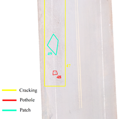
From the orthomosaic, AutoCAD® 2018 software vectorized each element to manually classify the pathologies (Fig. 1).
 |
||||
| Figure 1. Example of manual delimitation of pathology areas. | ||||
To obtain reference data for the survey carried out with the RPA, pathologies were evaluated by path, identifying the type and extent of the pathologies to verify whether the existing pathologies on the road would be visible in the images obtained by the RPA.
2.3 Supervised classification of images
A complement to the QGIS platform (Quantum Geographic Information System), the SCP (Semi-Automatic Classification Plugin) allowed the application of the supervised classification of images. From the final orthoimage, the plugin created a set of bands equivalent to the pre-processing step. The first processing stage includes the following categories: asphalt pavement in good condition, cracks, potholes, patches, vegetation (overlapping the road), and areas with clayey material. Next, samples of each element of interest to the classification were selected, which may have a pixel or a polygon as a capture instrument. These samples feed the training file, obtaining a raster image as a result of the classification.
In order to estimate the most appropriate supervised classification method for the machine used, the tests included combinations of variables associated with the identification criteria per pixel or polygon of the classification algorithm (minimum distance, maximum distance, maximum likelihood, or spectral angle mapping) and the number of samples for machine learning.
Four samples of each element were randomly collected for the first test, eight for the second, and sixteen for the third, totaling 24, 48, and 96 samples, respectively. This stage allowed a choice of samples consistent with the machine's capacity. Using the SCP, samples were collected by pixel, where the area with pixels similar to the selected one is delimited, and by polygon, where the area is delimited manually (Fig. 2).
 |
||||
| Figure 2. Examples of sampling by polygon (a) and by pixel (b) | ||||
As for image classification algorithms, SCP provides three options: (1) Minimum Distance, which classifies pixels by the average spectral distance between categories, by Euclidean distance, according to Eq. (1) (Richards, 2013):

Where d(x,y) is the Euclidean Distance, xi : Spectral signature vector of the pixel image, yi : Spectral signature vector of the area of a sample, n: Number of bands in the image.
(2) Maximum Likelihood, which calculates the normal probability distribution of the class, according to Eq. (2) (Richards, 2013):

Where g k x is the Normal Probability Distribution of the class, x: Spectral signature vector of the pixel image, C k : Land cover class k, p ( C k ) : Probability that the correct class is C k , | Σ k |: Determinant of the covariance matrix of data in class C k , Σ k - 1 : Inverse of the covariance matrix, y k : Spectral signature vector of class k.
(3) Spectral Angle Mapping, which determines the degree of similarity between spectral curves, according to Eq. (3) (Kruse et al., 1993):

Where θ x , y is the spectral angle, x i : Spectral signature vector of the pixel image, y i : Spectral signature vector of the area of a sample, n: Number of bands in the image.
The several combinations of identification criteria, classification algorithms, and number of samples allowed us to choose the best ones for this study. The results with the highest percentage of correct answers regarding the type and extent of pathologies were obtained with the Maximum Likelihood classifier using the polygon method with 24 and 48 samples. This study discarded tests with more samples due to the machine's capacity and the program's operating mode, which, during processing, continually overload the machine's memory.
2.4 Comparative and statistical analysis
After comparing the manual classification of images with data from the walking survey, manual classification was considered a reference for supervised classifications due to the high conformity of manual classification with pathologies in the field.
The Kappa index, a multivariate statistical technique, allowed for the assessment of the classifier's accuracy in identifying pathologies. The study compared the supervised classification with the samples used for training the algorithm and the supervised classification with the manual one. The Kappa indices obtained results from the Error Matrix (or confusion) provided in QGIS post-processing and the Manual versus Supervised Success Matrix, respectively. In addition to this, another parameter used for class analysis was the Matthews Correlation Coefficient (MCC).
2.4.1 Comparison of supervised classification successes with manual classification
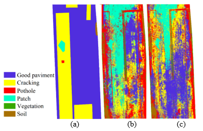
With the aid of QGIS, the polygons obtained in the manual classification were superimposed on the polygons from the supervised classification, resulting from transforming of the raster image into polygons. Thus, the study obtained common area of both classifications for each element. To verify the percentage of correct pathology identification, the manual classification results were confronted with those of the supervised classification from 24 and 48 samples. As an example, Figure 3 shows the same section manually classified (a) and supervised, with 24 samples (b) and 48 samples (c).
 |
||||
| Figure 3. (a) Manual, (b) Supervised with 24 samples and (c) Supervised with 48 samples. | ||||
2.4.2 Confusion Matrix
The confusion matrix compared the prediction class values for the validation data to the known values (Story; Congalton, 1986; Campbell; Hall-Beyer, 1997). This matrix maps the actual values of the validation set classes along the columns against the classes predicted by the classifier in the rows. The matrix diagonal displayed the correctly classified pixels, while cells outside the diagonal displayed those classified incorrectly or confused with another class (Mcgwire; Fisher, 2001).
True positives (TP) and true negatives (TN) are the correct classifications. A false positive (FP) occurs when the outcome prediction is incorrect, such as yes (or positive) when it is no (negative). A false negative (FN) occurs when the prediction of the result is negative when the true result is positive (Witten; Frank; Hall, 2016). From these frequencies, classification performance indicators reflect the classifier's efficiency in detecting a given class. A multiclass confusion matrix (k x k), like the one in the case under study, can be represented as a set of k binary confusion matrices, one for each class, allowing further processing (Ruuska et al., 2018).
2.4.3 Kappa Statistics
In 1960, Jacob Cohen created the Kappa (K) index to measure the precision or degree of agreement between predicted and observed categorizations of a data set (Cohen, 1960). The coefficient also indicates the degree of agreement between the supervised classification and the reference data, which can be the samples used in training the classification algorithm or an image of the manual classification defined as correct. In maps, the degree of agreement of the Kappa index can vary between 0 and 1, and the closer to the unit, the greater the degree of agreement. The interpretation of the classification proposed by Landis and Koch (1977) is used here, represented in Table 1:
| Table 1. Level of agreement based on the Kappa index | |||||||||||||||||||
| Kappa value | Interpretation | ||||||||||||||||||
|---|---|---|---|---|---|---|---|---|---|---|---|---|---|---|---|---|---|---|---|
| 0,00 - 0,20 | Minimal | ||||||||||||||||||
| 0,21 - 0,40 | Weak | ||||||||||||||||||
| 0,41 - 0,60 | Moderate | ||||||||||||||||||
| 0,61 - 0,80 | Strong | ||||||||||||||||||
| 0,81 - 1,00 | Almost Perfect | ||||||||||||||||||
| Source: Adapted from Landis and Koch (1977). | |||||||||||||||||||
Equation 4 calculates the Kappa index (K):

Po is the proportion of observed agreement, or overall accuracy, and 푃 푐 is the proportion of casual agreement or total acceptance. The Division 5 gives the term PO:

TP is the number of true positives, TN is the number of true negatives, and n is the total number of classified pixels. Equation 6 gives the term P C :

Where PC is the total number of pixels classified in each class, PCR is the total number of pixels in the actual class, and n² is the square of the total pixels.
2.4.4 Matthews Correlation Coefficient
The Matthews correlation coefficient (MCC) was first used by Matthews (1975). According to Baldi et al. (2000) MCC measures the quality of classifications. Their values range from -1 to +1, where coefficients closer to +1 represent a consistent forecast, those closer to 0 represent completely random forecasts, and those closer to -1 represent an inconsistent forecast. Eq. (7) calculates MCC:

TP is the number of true positives, TN is the number of true negatives, FP is the number of false positives, and FN is the number of false negatives. Pixels from different categories can result in similar spectral values and cause misclassification. Therefore, it is essential to indicate the classifier's performance in detecting a given class, and the MCC fulfills this role through the binary matrix of each category.
3. Results and discussion
Four topics present the results: (i) flight performance and processing, (ii) manual classification of images, (iii) supervised classification of images, and (iv) comparison of methods and statistical analysis of supervised classification.
3.1 Flight and processing
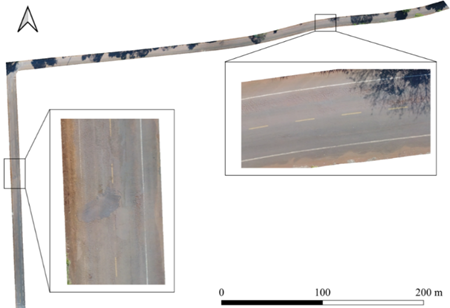
After performing the flight and processing the images obtained in the RPA survey, a final orthomosaic was generated (Fig. 4). The GSD was 1.39 cm per pixel. To optimize the classification, we cut out of the image the excess edges that contained the surroundings beyond the limits of the track lane.
 |
||||
| Figure 4. Final orthoimage. | ||||
3.2 Manual image classification
Manual classification of pavement surface pathologies was relatively quick due to the ease of identification from orthoimaging. On the other hand, after a subsequent check with the survey by walking, it was evident that the shadows of trees adjacent to the road made it difficult to visualize some pathologies and their extent, mainly cracks. In addition, vegetation hid parts of the pavement.
RPA images did not identify five pathologies noted in the walking survey. The area of patches, potholes, and cracks observed in the collection by walking was 1,759.45 m², while in the manual survey, it was 1,638.42 m², resulting in the identification of 93.1% of pathologies. The percentage was calculated based on geometric measurements recorded in sketches, with scale, in the walking survey.
3.3 Supervised classification of images
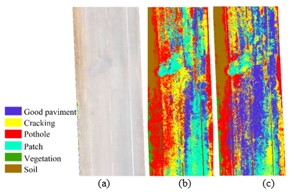
The classification of samples by polygons showed few regions in agreement with the actual surface condition of the pavement, as shown in Fig. 5. In addition, it resulted in different classifications for most of the selected image elements.
 |
||||
| Figure 5. (a) Pavement, (b) classification by polygons with 24 samples and (c) 48 samples. | ||||
Pixels from different categories, such as good pavement and patches, presented similar shades in some images, resulting in similar spectral values and, consequently, in classification errors. The results found that some errors occurred due to shading and overlapping vegetation, making it impossible to classify these locations.
3.4 Comparative and statistical analysis
In this topic, we present confusion matrices and scatter plots generated from the confusion matrix resulting from the relationship between manual and supervised classifications. These results allowed calculating the Kappa index (K) and the Matthews Correlation Coefficient (MCC).
3.4.1 Comparison between manual and supervised classifications
For the comparison of manual and supervised classifications, Tab. 2 presents the results of the Maximum Likelihood method through identification by polygon with 24 and 48 samples, including identified areas and percentages of correct answers.
| Table 2. Results of the Comparison between Manual and Supervised Classification. | ||||||||||||||
| Classes | Manual | Superv. 48 samples | Superv. 24 samples | |||||||||||
|---|---|---|---|---|---|---|---|---|---|---|---|---|---|---|
| Areas (m2) | Areas (m2) | Acerto (%) | Areas (m2) | Acerto (%) | ||||||||||
| Good paviment | 4419.39 | 1233 | 27.9 | 1346.67 | 30.47 | |||||||||
| Cracking | 1552.5 | 458.76 | 29.55 | 467.19 | 30.09 | |||||||||
| Pothole | 2.53 | 1.24 | 49.01 | 0.66 | 26.09 | |||||||||
| Patch | 83.39 | 25.73 | 30.86 | 42.12 | 50.51 | |||||||||
| Vegetation | 247.4 | 186.14 | 75.24 | 192.52 | 77.82 | |||||||||
| Soil | 29.45 | 22.2 | 75.38 | 20 | 67.91 | |||||||||
| Total | 6334.65 | 1927.06 | 30.42 | 2069.16 | 32.66 | |||||||||
The supervised classification with 24 and 48 samples resulted in an overall hit percentage of 32.66% and 30.42%, respectively. This result indicates that the number of samples needed is more relevant for accurately classifying areas with or without pathologies.
3.4.2 Confusion matrices and scatterplots
Tabs 3 and 4 represent classification error matrices. 'Px', 'Pav', and 'class' refer to Pixels, Pavement good, and Classifieds, respectively. Rows contain sorted data, while columns contain reference data. Internal values represent the pixels, and correctly identified pixels were highlighted.
| Table 3. Classifier confusion matrix with 24 samples. | ||||||||||||||
| Pav. | Crack | Pothole | Patch | Vegetation | Soil | Px class | ||||||||
|---|---|---|---|---|---|---|---|---|---|---|---|---|---|---|
| Pav. | 48682 | 9749 | 148 | 726 | 430 | 59735 | ||||||||
| Cracking | 3722 | 61794 | 123 | 667 | 1458 | 67764 | ||||||||
| Pothole | 307 | 5885 | 489 | 222 | 1150 | 755 | 8808 | |||||||
| Patch | 9887 | 13114 | 24 | 12162 | 182 | 35369 | ||||||||
| Vegetation | 34 | 97 | 39 | 62564 | 207 | 62941 | ||||||||
| Soil | 19 | 3 | 7 | 61161 | 61190 | |||||||||
| Px reais | 62632 | 90658 | 787 | 13816 | 65791 | 62123 | 295807 | |||||||
| Table 4. Classifier confusion matrix with 48 samples. | ||||||||||||||
| Pav. | Crack | Pothole | Patch | Vegetation | Soil | Px class | ||||||||
|---|---|---|---|---|---|---|---|---|---|---|---|---|---|---|
| Pav. | 190051 | 12879 | 450 | 1130 | 551 | 11 | 205072 | |||||||
| Cracking | 18926 | 55103 | 785 | 1757 | 299 | 76870 | ||||||||
| Pothole | 2367 | 4299 | 2354 | 1183 | 312 | 89 | 10604 | |||||||
| Patch | 9549 | 5383 | 229 | 12819 | 21 | 28001 | ||||||||
| Vegetation | 402 | 88 | 15 | 2 | 35516 | 17 | 36040 | |||||||
| Soil | 309 | 12 | 44 | 26 | 6725 | 7116 | ||||||||
| Px reais | 221604 | 77764 | 3877 | 16891 | 36725 | 6842 | 363703 | |||||||
The overlapping polygons defined in the manual and supervised classifications verified the correspondence of the identified pathologies. Figures 6 and 7 show the scatter plots of the percentage of pathologies identified by class for 24 samples (Figure 6) and 48 samples (Figure 7) derived from the confusion matrices for these cases.
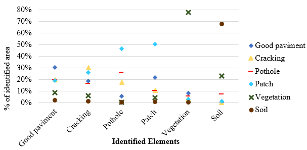 |
||||
| Figure 6. Dispersion of assertiveness: supervised classification 24 samples x manual | ||||
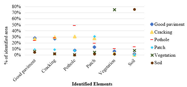 |
||||
| Figure 7. Dispersion of assertiveness: supervised classification 48 samples x manual | ||||
Fig. 6 shows that the land and vegetation classes presented better results, with percentages of correct answers more significant than 60 and 70%, respectively. Good pavement, cracks, and patches presented values between 30 and 50%, understood as a bad result. The pans present the worst result, with a hit of approximately 25% and a higher number of areas erroneously classified as patches.
Fig. 7 shows that the percentages of correct answers were similar to those in Fig. 6a, but with a significant increase for the pans. The Maximum Likelihood algorithm applies maximum likelihood (MaxVer), which explains these results. According to INPE (2006), the method weights the distance between the average values of the element's pixels through statistical parameters, assuming that all bands have a normal distribution, and calculates the likelihood that a pixel belongs to a specific element based on the samples. Thus, since the pot class presents different characteristics in the same occurrence, more samples contributed to a higher percentage of correct answers for this classifier.
3.4.3 Kappa statistic
The study calculated the Kappa index for four scenarios in two different comparisons. The first and best-known refers to the degree of agreement between categories predicted by the supervised classification for 24 and 48 samples for the data obtained in loco. The second consists of the degree of agreement between supervised and manual classification, referring to the visual identification and manual delimitation of pathologies. This analysis aims to elucidate the relevance of the Kappa index for analyzing pathologies in pavements through RPA based on the supervised classification of images. Table 5 shows the Kappa indices calculated from the confusion matrices presented in item 3.4.2.
| Table 5. Kappa indices for the four cases. | ||||||||||||||
| Matrix Used | 24 samples | 48 samples | ||||||||||||
|---|---|---|---|---|---|---|---|---|---|---|---|---|---|---|
| Supervised classification | 0.791 | 0.718 | ||||||||||||
| Overlapping manual and supervised ratings | 0.378 | 0.396 | ||||||||||||
According to the classification by Landis and Koch (1977), the indices of both classifiers are between 0.61 and 0.80, characterized as good agreement. However, for the correct classification by superimposing manual and supervised classifications, the Kappa values range from 0.21 to 0.40, corresponding to weak agreement.
The discrepancy between Kappa values obtained by the classifier and overlapping manual and supervised classifications shows that the index is not convenient for the qualitative analysis of pathologies from RPA despite being widely used in remote sensing. Quantitatively, the algorithms presented concordance was classified as good. However, they did not faithfully represent the positions and geometries of the pathologies, which can lead to erroneous interpretations regarding the accuracy of the assessment and, consequently, in decision-making regarding maintenance and rehabilitation strategies for the pavements.
3.4.4 Matthews Correlation Coefficient (MCC)
Due to the spectral similarity of the elements involved in the classification process, the MCC analyzed the classifier's performance for 24 and 48 samples of each class (Tab. 6).
| Table 6. Matthews Correlation Coefficient was obtained for each class. | ||||||||||||||
| Class | 24 samples | 48 samples | ||||||||||||
|---|---|---|---|---|---|---|---|---|---|---|---|---|---|---|
| Good Pav. | 0.74 | 0.72 | ||||||||||||
| Cracking | 0.71 | 0.63 | ||||||||||||
| Pothole | 0.18 | 0.35 | ||||||||||||
| Patch | 0.52 | 0.56 | ||||||||||||
| Vegetation | 0.96 | 0.97 | ||||||||||||
| Soil | 0.99 | 0.96 | ||||||||||||
Sorting results for 24 and 48 samples were similar. The potholes resulted in more classification errors because they have different colors, sometimes shaded or with clayey material. The patch element presented MCCs from 0.52 to 0.56, while "crack" and "good pavement" presented MCCs above 0.6 and 0.7, respectively, indicating that cracks have more significant potential for automated classification.
4. Conclusion
The study points out that identifying asphalt pathologies by RPAs can be an alternative to the traditional survey by walking, being more agile and safer, and not interrupting local traffic. The good level of detail of the images allowed a reliable manual classification (93.1% accuracy) in the visual identification and representation of the pathology's perimeter (extension) when taking as reference the data recorded in walking surveys.Supervised classification based on RPA is more complex than evaluation by walking, as it depends on specific equipment, adequate planning of flight plans, and reliable classification techniques and algorithms. The number of training samples was irrelevant, but how each sample was selected was decisive and should be standardized and carried out in such a way that the training of the algorithm is satisfactory.The Kappa indices, obtained by superimposing the images of the manual and supervised classifications, must be used with caution for the classification accuracy analysis because, without considering the location, verified here by superimposing the pathologies and verifying the type and extension of each target element, they can lead to mistaken interpretations about the assertiveness of the classification and, consequently, the condition of the pavements.
The results obtained from complementary analyses indicate that the supervised classification did not show the desired accuracy for applications aimed at pavement management, as it does not characterize pathologies in detail about type, location, and extent when compared to the in-loco survey and manual classification of images. As a result, we recommend that, in future studies, image treatment techniques be used that include the combination of pixel coloring, pathology geometry, and image pre-treatment, in addition to the application of other algorithms and processing techniques that allow the use of a more significant number of samples for training.
References
Astor, Y., Nabesima, Y., Utami, R., Sihombing, A. V. R., Adli M. and Firdaus M. R. (2023), Unmanned aerial vehicle implementation for pavement condition survey. Transportation Engineering. 12(2023):100168. https://doi.org/10.1016/j.treng.2023.100168
Baldi, P., Brunak, S., Chauvin, Y., Andersen, C. A. F., Nielsen, H. (2000), Assessing the accuracy of prediction algorithms for classification: An overview. Bioinformatics, 16(5), 412-424. https://doi.org/10.1093/bioinformatics/16.5.412
Branco, L. H. C., Segantine, P. C. L. (2015), “MaNIAC-UAV - A methodology for automatic pavement defects detection using images obtained by Unmanned Aerial Vehicles”. Journal of Physics: Conference Series, 633(1). https://doi.org/10.1088/1742-6596/633/1/012122
Campbell, J. B., Hall-Beyer, M. (1997), “Introduction to remote sensing”. Cartographica, Toronto, Canadá, p. 70.
Cohen, J. (1960), A coefficient of agreement for nominal scales. Educational And Psychological Measurement, 10(1):37-46. https://doi.org/10.1177/001316446002000104
Kruse, F. A., Lefkoff, A. B., Boardman, J. W., Heidebrecht, K. B., Shapiro, A. T., Barloon, P. J., Goetz, A. F. H. (1993). “The spectral image processing system (SIPS)- interactive visualization and analysis of imaging spectrometer data” in: AIP Conference Proceedings 283, Pasadena: California (USA), pp. 145-163. https://doi.org/10.1063/1.44433
Hassan, S.-A., Rahim, T., Shin, S.-Y. (2021), An improved deep convolutional neural network-based autonomous road inspection scheme using unmanned aerial vehicles. Electronics. 10(22):2764. https://doi.org/10.3390/electronics10222764
INPE. Manual de Geoprocessamento. Disponível em: <http://www.dpi.inpe.br/spring/portugues/tutorial/introducao_geo.html>. Acesso: 8 out. 2021.
Landis, J. R., Koch, G. G. (1977), The Measurement of observer agreement for categorical data. Biometrics, 33(1):159-174. https://doi.org/10.2307/2529310
Matthews, B. W. (1975), Comparison of the predicted and observed secondary structure of T4 phage lysozyme. Biochimica et Biophysica Acta, 405(2):442-451. https://doi.org/10.1016/0005-2795(75)90109-9
McGwire, K. C., Fisher, P. (2001), Spatially Variable Thematic Accuracy: Beyond the Confusion Matrix. Spatial Uncertainty in Ecology, 308-329. https://doi.org/10.1007/978-1-4613-0209-4_14
Oliveira, F. H. L. de, Arantes, A. E., Lima Neto, P. D. S. (2020), Estudo de método para identificação de panelas e remendos em pavimentos urbanos com a utilização de UAS quadrirrotor. Revista Tecnologia, 41(2):1-14. https://doi.org/10.5020/23180730.2020.10838
Pan, Y., Zhang, X., Cervone, G., Yang, L. (2018), Detection of Asphalt Pavement Potholes and Cracks Based on the Unmanned Aerial Vehicle Multispectral Imagery. IEEE Journal of Selected Topics in Applied Earth Observations and Remote Sensing, 11(10):3701-3712. https://doi.org/10.1109/JSTARS.2018.2865528
Parente, D. C., Felix, N. C., Picanço, A. P. (2017), Utilização de veículo aéreo não tripulado (VANT) na identificação de patologia superficial em pavimento asfáltico. Revista ALCONPAT. 7(2):160-171. https://doi.org/10.21041/ra.v7i2.161
Pinto, L., Bianchini, F., Nova, V., Passoni, D. (2020), Low-Cost UAS Photogrammetry for Road Infrastructure's Inspection. International Archives of the Photogrammetry, Remote Sensing and Spatial Information Sciences - ISPRS Archives, 43(B2):1145-1150. https://doi.org/10.5194/isprs-archives-XLIII-B2-2020-1145-2020
Ragnoli, A., De Blasiis, M. R., Di Benedetto, A. (2018), Pavement distress detection methods: A review. Infrastructures, 3(4):1-19. https://doi.org/10.3390/infrastructures3040058
Ranjbar H., Forsythe, P., Fini, A. A. F. and Maghrebi M. (2023), Addressing practical challenge of using autopilot drone for asphalt surface monitoring: road detection, segmentation, and following. Results in Engineering. 18(2023):101130. https://doi.org/10.1016/j.rineng.2023.101130
Ranyal, E., Sadhu A., Jain K. (2022), Road condition monitoring using smart sensing and artificial intelligence: a review. Sensors. 22(8):3044. https://doi.org/10.3390/s22083044
Richards, J. A. (2013), “Remote Sensing Digital Image Analysis”. Springer-Verlag Berlin Heidelberg, 5ed., Heidelberg, Alemanha, p. 340. https://doi.org/10.1007/978-3-642-88087-2
Ruuska, S., Hämäläinen, W., Kajava, S., Mughal, M., Matilainen, P., Mononen, J. (2018), Evaluation of the confusion matrix method in the validation of an automated system for measuring feeding behaviour of cattle. Behavioural Processes, 148:56-62. https://doi.org/10.1016/j.beproc.2018.01.004
Schnebele, E., Tanyu, B. F., Cervone, G., Waters, N. (2015), Review of remote sensing methodologies for pavement management and assessment. European Transport Research Review, 7(2):1-19. https://doi.org/10.1007/s12544-015-0156-6
Shaghlil, N., Khalafallah, A. (2018), “Automating Highway Infrastructure Maintenance Using Unmanned Aerial Vehicles” in: Construction Research Congress 2018, New Orleans: Louisiana (USA), pp. 486-495. https://doi.org/10.1061/9780784481295.049
Story, M., Congalton, R. G. (1986), Remote Sensing Brief - Accuracy Assessment: A User’s Perspective. Photogrammetric Engineering and Remote Sensing, 52(3):397-399. doi: 0099-1112/86/5203-397$02.25/0
Tan, Y., Li, Y. (2019), UAV photogrammetry-based 3D road distress detection. ISPRS International Journal of Geo-Information, 8(9):409. https://doi.org/10.3390/ijgi8090409
Witten, I. H., Frank, E., Hall, M. A. (2016), “Data Mining - Practical Machine Learning Tools and Techniques”. Morgan Kaufmann Elsevier, Burlington, pp. 654.
Zhu, Q., Dinh, T. H., Phung, M. D., Ha, Q. P. (2021), Hierarchical Convolutional Neural Network with Feature Preservation and Autotuned Thresholding for Crack Detection. IEEE Access, 9:60201-60214. https://doi.org/10.1109/ACCESS.2021.3073921
